All Excel’s Date and
Time Functions Explained!

When analyzing and manipulating date information in Excel, you have several formatting options.

In other words, you can display your data in many ways.

Most of the time, Excel will know that you are entering a date when you key in the data like the following:

• 1/1/2017
• January 1, 2017
• 1-Jan

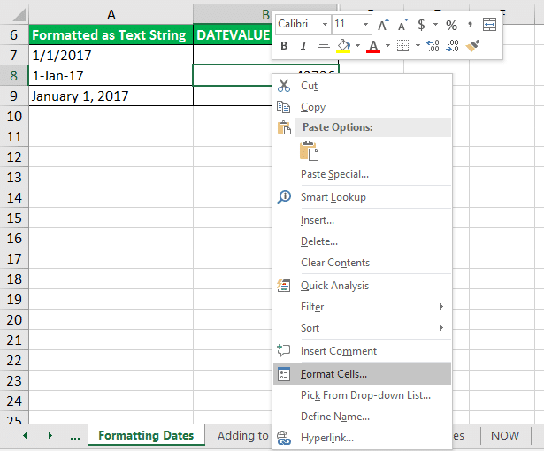
Below are a few examples of the various formats that Excel displays dates in.

But the key is that they are all aligned to the right of the cell.

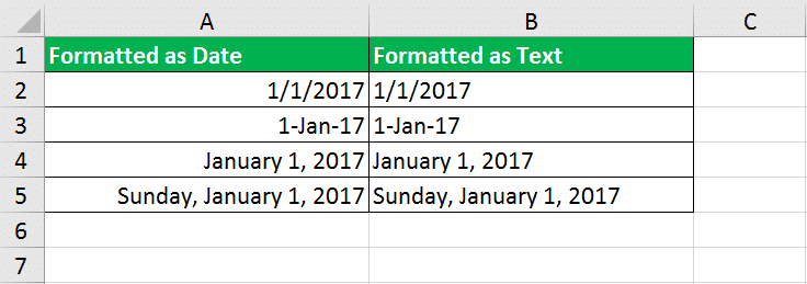
Contrast column A with column B (where the cells are formatted as text). They show the same information.

One important note about how Excel stores dates:

To use dates in calculations, Microsoft Excel stores dates as serial numbers.

These are the sequential number of the day in relation to the starting date of January 1, 1900.

So, think of January 1, 1900, as serial number 1.

January 1, 2016, would be serial number 42370 as it’s 42,370 days after January 1, 1900.

Now you know the fundamentals of date formatting versus date data formatted as text. Let’s look at some calculations you can do with dates.

How to add days to a date

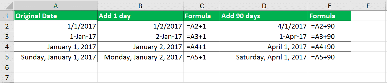
Adding days to a date is very simple, straightforward, and intuitive.

All you need to do is add the number of days as a single number to the date or cell reference containing the date.

The following figure illustrates just how simple it is to add 1 day or 90 days to a date.

How to add months to a date

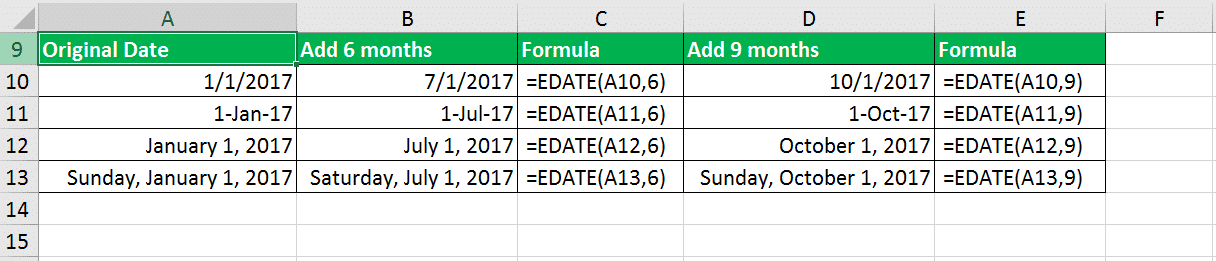
If you need to add a month or several months to your date, the process is a bit more complicated.

Here’s its syntax:

=EDATE(start_date, months)

The function requires 2 arguments: ‘start_date’ and ‘months’.

The first, ‘start_date’, is simply the date we are adding months to.

The second, ‘months’, is the number of months we would like to add to the date.

Look at the figure below to see just how easy it is to calculate a new date by adding 6 months and 9 months to the start date.

How to add years to a date

So, what about calculating the addition of years to your original date?

The first function we need to focus on is DATE.

The syntax for DATE is also incredibly simple and intuitive:

=DATE(year, month, day)

But, for our purposes, we can use the YEAR, MONTH, and DAY functions along with DATE.

These functions extract the correct data from our original date. This ensures appropriate use of our final DATE formula.

For example, applying MONTH to a cell reference of our original date will extract the month data. The same is true for YEAR and DAY.

That was a lot, so let’s look at the following figure to see it in action.

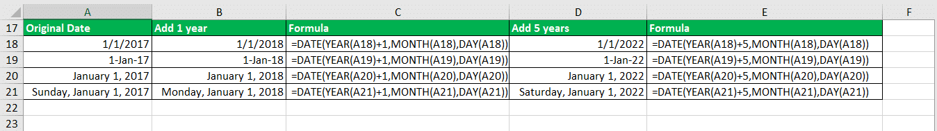
Notice row 18 and column C of the worksheet.

The ‘year’ argument of the ‘DATE’ function is substituted by the function ‘YEAR(A18)+1’.

This tells the DATE function that we want the year only from the date data in A18 (or 2017) – and that we want to add ‘1’ to it (or 2018).

Adding time to a date is super useful.

But what if you had a report where you needed to calculate the difference between dates?

Find the difference between two dates

To find the difference between two dates, we want to turn our attention to the DATEDIF function.

This requires you to type the formula in its entirety.

There will be no tooltip hint as you begin to type the function.

Let’s look at the syntax:

=DATEDIF(start_date, end_date, unit)

There are three arguments for the DATEDIF function:

• start_date: This is the initial date of the period among the two you are calculating the difference between.
• end_date: This is the latest date of the two.
• unit: This is the unit in which you want the function to return the difference by. More on units right below…

The ‘unit’ argument gives you a choice of several formats to return your results from DATEDIF.

• y – The number of complete years between dates.
• m – The number of complete months between dates.
• d – The number of days between dates.
• md – The number of days ignoring months and years.
• yd – The number of days ignoring years.
• ym – The number of months ignoring days and years.

In our example, you can use literal dates if they are enclosed in double quotes.

You can also use the serial number format as shown in rows 4 and 5.

But in the second example, we use ‘md’ for the unit argument. ‘md’ is the difference between the dates in days – ignoring the months and years. That is 15 minus 1, or 14 days.

You can also calculate the difference between two dates in cells.

To do this, place the cell reference of your dates in the ‘start_date’ and ‘end_date’ arguments.

One (last) important thing to note about using DATEDIF:

The ‘end_date’ argument must always be later than the ‘start_date’ or you will get the ‘#NUM!’ error.

Now let’s turn our attention to some tricks and shortcuts involving the current date.

Often, you need to work with the current (today’s) date.

There are some nifty tricks that allow you to do this without typing in the entire date manually.

Let’s look at them!

Use date that updates itself with the TODAY function

One of the simplest ways to input today’s date into a cell is to use the TODAY function.

Do this by typing ‘=TODAY()’ into a cell.

This places the current date into the cell dynamically. So, that cell would have tomorrow’s date in it if you reopen the file tomorrow.

Insert static current date in Excel using shortcuts

You can also insert the current date using keyboard shortcuts.

For the current date, press the following key combination:

Ctrl + ;

To insert both the date and the time, press the previous keyboard shortcut. Then press the following combination:

Ctrl + Shift + ;

These shortcuts enter static dates and times. This opposed to the dynamic date that the TODAY function returns.

Subtract a date from the current date

You can use the current date in a calculation like subtracting.

You replace the ‘start_date’ argument in the DATEDIF formula.

Above image shows how to substitute the TODAY function for a literal date value or cell reference for the ‘start_date’ OR the ‘end_date’.

Remember the rule that the ‘end_date’ must be later than the ‘start_date’ still applies.

You can also use the keyboard shortcut to insert the current date if you need to insert the static date. This is a quicker and more efficient way to insert today’s date.

There are often situations where you need to retrieve numbers from dates.

But, you might not have the need for an entire date.

Let’s say you have a report. Here you want to separate the different elements of the date for filtering by a single element of the date – like the month or year.

Here’s how to go about doing that 🙂

Use the DAY function to find the day of a date

To isolate only the day of the full date, we use the DAY function.

There is a single argument for the DAY function:

=DAY(serial_number)

You probably know by now that ‘serial_number’ is the date.

This argument can be the actual serial number form of the date or the literal date in double quotes. It can also be a cell reference like in the following example.

Look at above picture again. Notice that regardless of the format of your original date, the DAY function returns the value ‘14’.

Use the MONTH function to find the month of a date

If you need to isolate the number value for the month of your original date, you can use the MONTH function.

It works the same way the DAY function works:

=MONTH(serial_num)

Use the YEAR function to find the year of a date

Now we move onto the function that retrieves the number value for the year part of the date.

The syntax for the ‘YEAR’ function is like the DAY and MONTH functions syntactically.

=YEAR(serial_num)

You already know how to retrieve the day and month number values. It’s the exact same concept when using the ‘YEAR’ function.

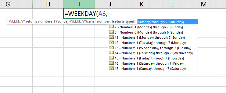
Use the WEEKDAY function to find the day of the week

You can also retrieve the number value for the day of the week from a date.

Here’s its syntax:

=WEEKDAY(serial_num, [return_type])

The syntax for WEEKDAY requires the ‘serial_number’ argument.

It also allows for an optional argument: ‘return_type’.

This allows you to choose a different start and end date for your week.

That means that the returned value will align with that chosen sequence.

Below you can see the list of different ‘return_type’ values that Excel allows.

In the following examples, note the value differences returned by the formula based on the ‘return_type’ argument.

The different selections for the ‘return_type’ in the formulas return very different weekday values.

These depend on the first day of the week that corresponds to those ‘return_type’ values.

Use the WEEKNUM function
to find out the week number

Another interesting built-in function is the WEEKNUM function.

WEEKNUM retrieves the number value for the week of the year that the original date falls within (1 – 52).

So, if the original date is between January 1 and January 7, the WEEKNUM value would be ‘1’.

If the date is between December 25 and December 31, WEEKNUM would return the value ‘52’.

=WEEKNUM(serial_number, [return_type])

Our date falls on a Monday.

The result of the WEEKNUM formula will be different if the ‘return_type’ argument is ‘1’ (Sunday) versus ‘12’ (Tuesday).

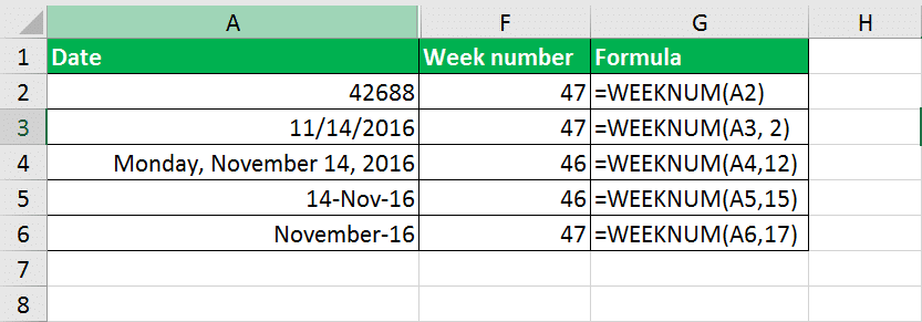
This can be a very useful function.

Consider a situation in which you needed a weekly countdown. Simply calculate the difference between dates using the WEEKNUM function.

Use the WORKDAY function to calculate the number of working days between two dates

Another useful function is the WORKDAY function.

This function returns a day that is some number of workdays into the future or before some date. A “workday” is days excluding weekends and any holidays that are specified.

The function requires two arguments and has an optional third.

=WORKDAY(start_date, days, [holidays])

• start_date – this required argument is the date from when you want to count the number of workdays
• days – this required argument is the number of days from the start date you want a count of. Using a negative number will give you the date that many workdays before your start date.
• holidays – this argument is optional. This allows you to add holiday dates in the formula for the WORKDAY function to skip along with weekends.

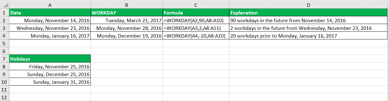
First, note that we have listed 3 holiday dates in cells A8, A9, and A10. We will be using these in our examples for the ‘holiday’ argument to exclude along with weekends.

On row 2, we want to know the date that is 90 workdays from Monday, November 14, 2016.

Excluding the weekends and holidays (A8:A10), this will be Tuesday, March 21, 2017 according to the WORKDAY function.

On row 3, we can instantly see the effect of weekends and holidays on the outcome of our formula. We want the date that is 2 workdays from Wednesday, November 23, 2017.

Because of the holiday on Thursday, November 24 – and the weekend days Saturday and Sunday – the result is Monday, November 28, 2016.

The third example in the figure illustrates how to use WORKDAY to find a date before the start date.

We want to know the date that is 20 workdays before Monday, January 17, 2017.

So, our DAY argument needs to be a negative value (-20).

Again, note the result considers weekend days as well as a couple of holidays.

In this section, we are going to cover how to work with sequences of dates. This time by using the autofill capability of Microsoft Excel.

You can use Autofill in 2 ways.

The first is to double-click the fill handle. The fill handle is a small square that appears in the lower right corner of a highlighted cell.

The second option is to simply drag the handle to the desired cell. Note the fill handle for the highlighted cell in the following figure.

The fill handle also offers some more options.

Try to right-click and drag outside the selection a bit.

We will focus on the selections that fill elements of the date like days, weekdays, months, and years.

Insert dates that increase by one day

To insert dates that increase by one day in a column, you can simply grab the fill handle.

Then drag it down as many rows as you need dates for.

One thing to take note of is that as you do this, Excel shows the incremented date as you drag the range.

So, you can see just what date you are at as you expand the range.

Once you release the fill handle, your range is now filled with dates.

These dates increment in one-day intervals.

Insert dates that increase by weekdays

But what if you wanted to increment a wide range of dates by weekdays only?

This is easily done by selecting ‘Fill Weekdays’ from the ‘Autofill Options’ that appears once you fill the dates down.

Once you select ‘Fill Weekdays’, Excel automatically excludes any weekend dates from the range.

Insert dates that increase by months and years

You can also use the ‘Autofill Options’ to increase months and years.

Select the fill option you need once you fill the dates down to the last cell of your range.

Insert dates that increase by several days

I’m sure you can think of other custom intervals (dates) you might like to fill down your column (or row, for that matter).

Microsoft Excel allows for a little of that also.

So, what if you wanted to increment every other day? Or what about every 3 months?

Click on ‘Series…’. The Series dialog box will now open.

This gives you several options for customizing the intervals of your dates.

For our example of every other day, you can select a Step value of ‘2’.

Leave everything else as it is.

In the beginning of this tutorial, I told you about the differences between text format and date format.

Also, remember our point earlier, that Excel stores date data as serial number.

So, no matter what date format you choose, Excel still recognizes it as a serial number.

What is date formatting?

Date formatting offers you choices on how you want to represent the date data in your worksheets.

Let’s look at our original example at the beginning of this tutorial.

We can see in the Number group of the Home tab that our data cells are all formatted as Date.

If you take the same data and place it into another column, something interesting happens.

In the cells that are formatted as ‘General’, you’d see the dates serial numbers.

If you run into this in your own spreadsheets, you must know how to fix this…

It’s quite simple, you just need to know how to reformat those cells into the Date format that you need.

For this example, let’s reformat to ‘Short date’.

Highlight the cell containing the serial number. Click on the drop-down arrow to see all the available formats in the Number group of the Home tab.

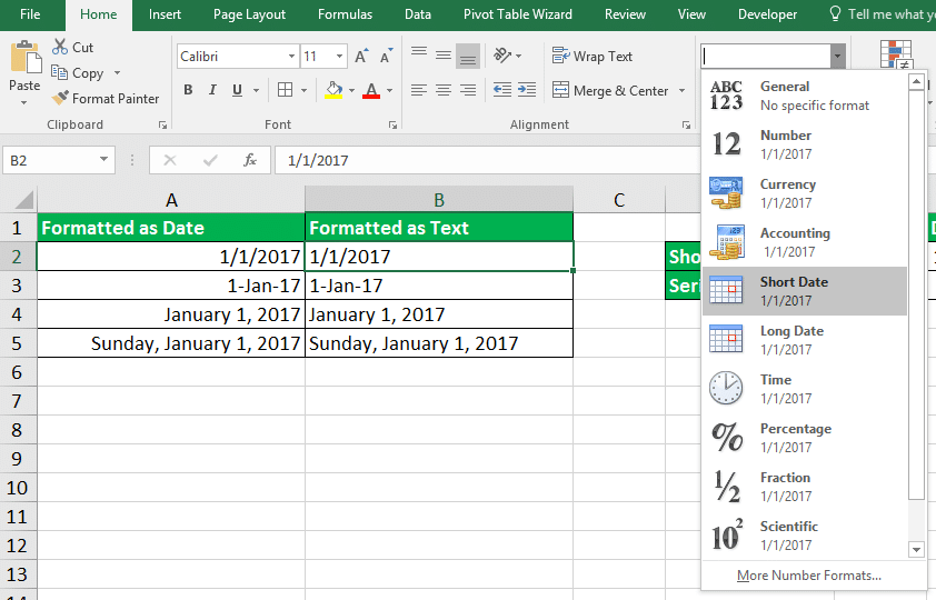
Select ‘Short Date’ from the dropdown and now the serial number will be converted from ‘General’ format to a date format that you recognize.

How to use other date formats
from the ‘Format Cells’ dialog box

You’ve now seen how to change date data formatted as ‘General’ to the ‘Short Date’ format.

Now we look at some other date formats that Excel also offers…

You already know how to change to a date format from the ribbon but you can also use the ‘Format Cells’ dialog box.

The first step is to find the cell that contains the serial number you want to reformat.

Then, right-click on the cell.

Select ‘Format Cells’ from the menu that appears.

From the Format Cells dialog box, select ‘Date’ in the Category box.

This reveals the different standard date format types available in Excel.

Decide on the ‘Type’ you want.

Then click ‘OK’ and the serial number now changes to the date format type you selected.

How to use custom date format

Even with all the date types Excel offers, you can still format your date data with your own custom format.

It is pretty simple to do…

Follow the same steps as we did with the previous example.

But, instead of choosing ‘Date’ in the Category box in the Format Cells dialog box, select ‘Custom’.

Take a second look at the picture above.

Here the Format Cells dialog box shows the current format of the cell in the Type and Sample boxes.

Let’s clear out the Type box…

And then type “mm-dd-yyyy”  into that box:

Turn text into dates with the DATEVALUE function

Another method for converting dates in text format is to use a function called DATEVALUE.

This function converts text string dates to their appropriate serial numbers.

The DATEVALUE syntax is simple:

=DATEVALUE(date_text)

So, let’s look at a few examples of cells containing dates that are in text string form.

Let’s use the DATEVALUE function in the column next to these cells.

Here it’s easy to see if the cells return the serial numbers we expect.

If your text date is before the year 1900, the DATEVALUE function will return the ‘#VALUE!’ error.

That’s because Excel recognizes dates as serial numbers beginning at January 1, 1900.

If your text date doesn’t contain a year, the DATEVALUE function defaults to the current year from your system clock.

How to auto populate date when a cell is updated

What if you wanted to make sure each time a cell’s data got updated, you knew when it was updated?

You could input the date and time manually in the cell next to it.

But what if you wanted to automate that process?

That way you’ll never forget to do it. Also, you would mitigate the chances for a data entry error.

A quick recommendation:

Excelribbon.tips.net has written an awesome guide that demonstrates a worksheet change event.

How to insert a date picker in Excel

Another cool thing you can do in Excel with dates is to create a date picker. This allows users to choose a date from a preset dropdown calendar. That way they don’t have to input the date by hand.

This is actually a pretty complex proposition in Excel. But if you want to see a date picker and a bit about how one can be created using VBA. Contextures has an amazing guide to do it right here.

Maybe you need to quantify elapsed time for tasks or projects?

Or perhaps you need to insert a time rather than a date in your data?

There are many parallels between the techniques of working with dates and time.

How to add time in Excel

Let’s look at a scenario where you have documented the total time it took for two different tasks in Excel.

Now you want to add those together to get your total time worked.

This is as simple as clicking on the cell below the task times and pressing Alt + = to autosum the times.

Now let’s look at a scenario where you have the times worked for a full workweek that you need to add together for a total.

If we autosum once again, we immediately notice a problem.

We know by simple inspection that these workday time values add up to more than 12 hours and 52 minutes.

What we need to do in our current situation is to right click on the cell where our auto sum formula is.

Then select Format Cells like we did with dates.

Then select ‘Custom’ from the Category box and clear the Type box.

Then in the Type box, type ”[h]:mm”.

Click ‘OK’ and you should have the correct total of hours for the week now.

How to find the difference between two times

Finding the difference between times is not quite as simple as adding times together.

Let’s look at a situation where we have a start time and an end time and we want to calculate the total elapsed time.

In cell B4, type the formula ‘=(B3-B2)*24’.

This subtracts the end time from the start time and then multiplies both by 24.

The multiplication by 24 is required since Excel recognizes times as a fraction of a full 24-hour day.

Our result is a numerical value and we choose to set it to two decimal places to show fractions of a full hour.

If you want to see the elapsed time in the actual hours and minutes, here’s what to do.

Remove the ‘*24’ and format using the custom format we created in the previous example adding times ([h]:mm).

Find current time in Excel

The NOW function allows you to insert the current time based on your computer’s system clock.

NOW returns the current date and time whereas TODAY returns the current date only.

But we can use NOW and format our cell so that it only shows the time but not the date.

Insert static current time with shortcuts

You’ve already seen the keyboard shortcut for entering in the static current date as well as entering the static current time.

Since we are discussing time data, I’ll show you how to use a keyboard shortcut to enter the static current time.

All you must do is press the following keyboard combination:

Ctrl + Shift + ;

Again, this contrasts with using the NOW function because it is static rather than dynamic.

This keyboard shortcut inserts the exact time you pressed the keyboard shortcut. It will remain that time unless you manually change it.

Retrieve seconds, minutes and hours

Let’s look at retrieving parts of time data.

This is very much the same as when you retrieved the month, day, and year, from dates. We are going to retrieve the seconds, minutes, and hours with some built-in functions available in Excel.

If you want to retrieve the seconds from a time value in Excel, you use the built-in SECOND function.

There is a single required argument for this function: ‘serial_number’.

=SECOND(serial_number)

Let’s look at a few simple examples to see this function in action:

For times that don’t display the seconds, the SECOND function still retrieves the seconds from the serial number of the date.

If you need to retrieve the minutes from your time data, you want to use the MINUTE function. Like with SECOND function (and others), there is only the required ‘serial_number’ argument.

=MINUTE(serial_num)

Now we will take the same time data we used for the SECOND function and use the MINUTE function.

The last thing we will look at is the HOUR function. Nothing new on the syntax.

=HOUR(serial_number)

One thing to note about the HOUR function is that it returns a value for the hour based on 24 hours.

So, if you want your HOUR function to return the hour in an AM/PM fashion, subtract 12 from your function if it is a time later than 12 PM.

Just like with dates, there are several different format types for time data.

In fact, our examples so far have demonstrated a few of these different formats.

You find the default time format types by right-clicking a cell.

Then select Format Cells.

Note in the figure above how many variations you can choose from. You can always create your own custom format by selecting ‘Custom’ from the Category list.

How to use and change time formatting

Now we have reviewed how you select different time formats.

Let’s look at a few examples of the different types.

We will look at 3 different selections from those available in the types for time formats.

The first thing we need to do to change format is to right click on the range of dates we want to reformat. Then select Format Cells.

Once the Format Cells dialog opens, select ‘Time’ from the Category box. Then in the Type box select ‘*1:30:55 PM’.

The asterisk in ‘*1:30:55 PM’ indicates that this format changes to the Region settings on your computer.

Any changes to the Windows time format settings will reflect in Excel. But only for the times formatted with a format preceded by an asterisk.

Turn text into time with the TIMEVALUE function

The DATEVALUE function converts dates in text string form to date formatting.

Like DATEVALUE, the TIMEVALUE function converts text string time data to actual time format.

See the syntax here:

=TIMEVALUE(text_time)

The ‘text_time’ argument is required. It is simply the text string date that you need to convert to time format.

So, when you use the TIMEVALUE function, you won’t get a time.

Rather, it returns a decimal number value that is a fraction of the entire day.

If you multiply the TIMEVALUE result by 24, you get a more accurate interpretation of the time (albeit still in decimal format).

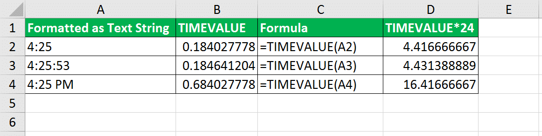
But if you reformat the TIMEVALUE result to a time format, you are good to go.

You will have changed a text string time to a true time format that Excel will now recognize as time instead of text.

There it is, the most comprehensive guide to date and time in Excel.

It’s taken us tons of hours and resources to publish. Feel free to share it along with anyone who needs to brush up their dates and times 😊

If you enjoyed this tutorial, I’m sure you’ll love this…