How to Not Calculate If Cell is Blank in Excel (Ignore Formula)

In Data Analysis, accounting for blank cells is a regular task. But sometimes, you might want to ignore these empty cells when applying a formula to a range.

It could be because the cell contains a null value that could result in an empty output. Or your main concern is the data entries and not the output values 🔢

Luckily, Excel offers different methods to ignore formulas in blank cells and focus on the data set. Let’s learn below how to not calculate value if a cell is blank in Microsoft Excel.

Download our free sample workbook here to get hands-on practice of the topic.

Table of Contents

How to Not Calculate Blank Cell Using IF Formula

The first method on how to not calculate empty cells uses an if function in the formula. Let’s see how this works below 🔽

The IF function to ignore blank cells is written as:

where,

range<>”” checks if the value in cell B2 is empty

[value_if_true],[value_if_false] work as the criteria to be fulfilled if the condition is met

Say, we have the following sample data.

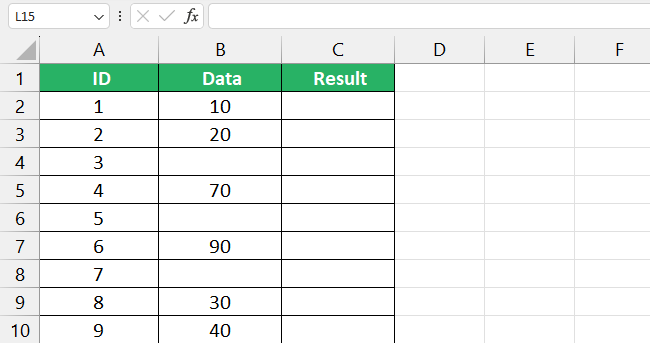
Step 1) Select cell C2.

Step 2) Type in the following formula.

Step 3) Press Enter.

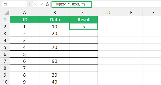
Step 4) Double-click the Fill Handle to copy the formula to the remaining cells in the range.

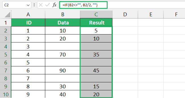
As visible, our condition applied the function to the cells with values inside them and retained the blank cell value – exactly what we wanted.

How simple is that? 😀

How to Not Calculate Blank Cell Using ISBLANK Function

You can also use the ISBLANK function to not calculate blank cells in Excel. It checks whether a cell is empty or not and like other IS functions, it returns boolean values of TRUE or FALSE.

The syntax of the ISBLANK function is given as:

where,

values refers to the cell you want to reference.

We will use a combination of Excel formulas – the ISBLANK function & IF function to ignore empty cells.

Say, we have the following sample data.

Step 1) Select cell C2.

Step 2) Enter the following formula

Step 3) Press Enter.

Step 4) Drag the Fill Handle down to copy the formula.

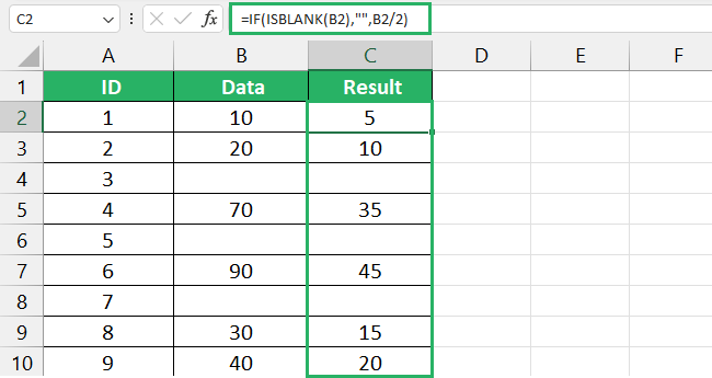
As evident, the formula checks the cells that are empty and goes to return blank cell.

See the image below for reference.

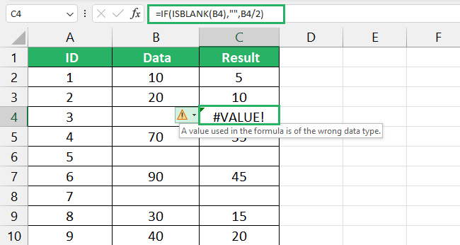
The error above is because cell B4 contains a space and is not empty.

How to Not Calculate Blank Cell Using COUNTBLANK Function

Another way to not calculate empty cells is to use the COUNTBLANK function in combination with the Excel IF function. Its syntax is pretty much the same as the ISBLANK function.

Let’s see it below.

Let’s see how to implement this formula now.

To do that,

Step 1) In column C, select cell C2.

Step 2) Type in the following formula

Step 3) Press Enter.

Step 4) Copy the formula to the remaining cells.

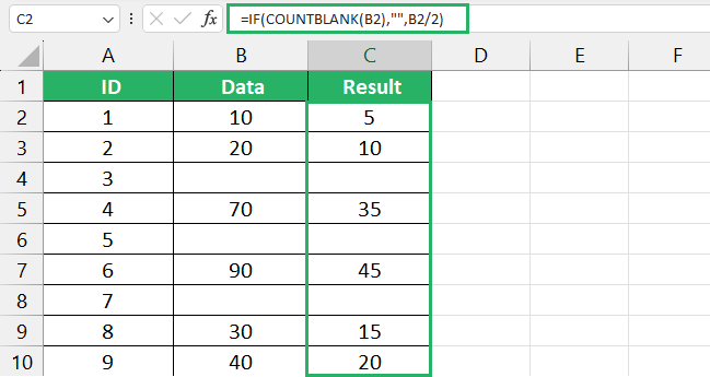
The COUNTBLANK function serves the same purpose as we saw with the simple IF and combination of ISBLANK and IF Excel functions.

Also, the COUNTBLANK function returns the same error as we saw earlier with the ISBLANK function which means that the blank cells in your range must be completely empty.

How to Not Calculate Blank Cell Using Conditional Formatting

In the above techniques we used, we had to apply different sorts of logic and complex formulas to get only the non-blank cells to return value.

But what if I told you there is an easier no-mathematical-fuss method to ignore blank cells in your worksheet? 📗

It’s the conditional formatting method where you apply a certain rule and Excel highlights the selected cells.

Let’s see how to do that below.

Say, we have the following sample data

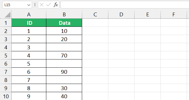
To use conditional formatting to highlight blank cells in your data range,

Step 1) Select the range of cells containing blank cells.

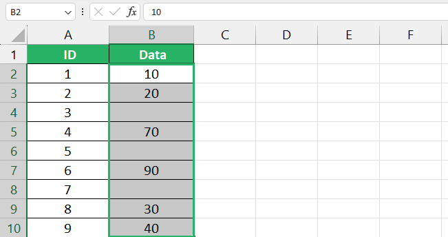
Step 2) Go to the Home tab.

Step 3) Click on Conditional Formatting.

Step 4) From the dropdown list, select New Rule.

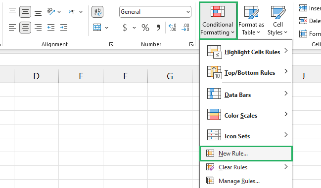
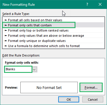
Step 5) A New Formatting Rule dialog box will appear on the screen.

Step 6) Select “Format only cells that contain” from the Rule Type.

Step 7) Click on the Format only cells with bar and select Blanks from the dropdown.

Step 8) Select Format in front of the Preview option.

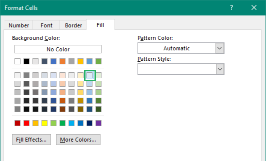
Step 9) Select the color you want your blank cells to be highlighted in from the Format Cells dialog box.

Step 10) Once done, press OK.

Empty cells in the selected range will be highlighted in the selected color.

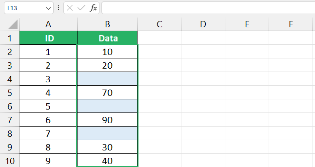
How cool is that? 😃

Conclusion

In this tutorial, we saw different methods of how to not calculate cells that were blank in a range. We used a simple IF formula, we also saw IF combined with different functions along with conditional formatting to highlight blank cells 🔲

Knowing this quick hack can make calculations much more flexible as you can copy data and share it into further analysis easily.

If you want to know more about Conditional Formatting in Excel, try reading these articles below:

How to Use Conditional Formatting to Highlight Text in Excel

How to Use the ISBLANK Function

We hope you enjoyed reading this article as much as we enjoyed creating this.