How to Use Conditional Formatting to Highlight Text in Excel

Conditional formatting in Excel is formatting that changes with the cell content.

That means you don’t have to change it when the cell content changes.

You use conditional formatting to make it easier for the user to identify key points of interest.

That could be:

• All cells that contain the name of a certain employee
• All rows regarding a certain order number

Or a lot of other things.

Follow this step-by-step guide and learn to highlight text with conditional formatting in Excel.

And a bit more😉

Download the workbook I use in this guide if you want to tag along.

Highlight text with conditional formatting

The reason for highlighting text with conditional formatting is to draw the user’s attention to those cells – so they find relevant information faster🏃

You apply conditional formatting with what is called conditional formatting rules.

It’s really easy to insert one of those.

1. Select all the cells where the text you want to highlight can be.

In the sample data, I want to identify all L compatible adapters. So, I select all cells in column B (from cell B2 and down).

2. In the middle of the Home tab, click ‘Conditional Formatting’.

3. Hover your cursor over ‘Highlight Cells Rules’ and select ‘Text that Contains’.

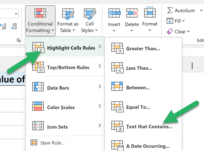
4. In the dialog box that appears, write the text you want to highlight, in the left field.

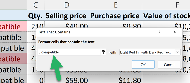
As you type it, you can see the conditional formatting applied instantly.

The formatting being applied is the standard conditional formatting format.

5. To change the format, click the drop-down arrow in the right field and select another of the formatting presets.

6. Or you can create your own format by clicking ‘Custom format’.

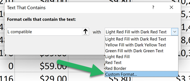
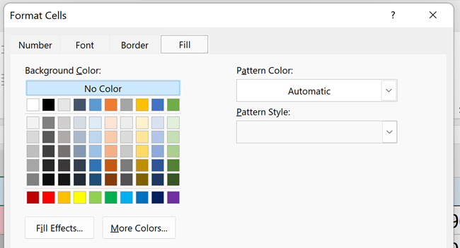
7. After clicking ‘Custom Format’ the ‘Format Cells’ dialog box appears.

This is the same as the normal ‘Format Cells’ dialog box you’re using when you apply normal formatting in a spreadsheet.

Use whatever formatting style you want for your conditional formatting rule.

And that’s it!

Now, all cells containing the text “L compatible” are highlighted with the chosen formatting.

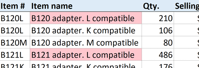
Pretty cool, right?💪

Highlight numbers with conditional formatting

Sometimes you’re not reading all your data in your sheets, you’re just looking for specific numbers.

That can be a tedious process, especially if you have a large data set.

Let’s dive into our inventory list again🤿

If the quantity in stock of an item reaches below 100 it’s critical that you find out, so you can buy more units of that particular item.

Let’s make a simple conditional formatting rule to highlight cells.

1. Select the cells in the quantity column (cells C2 and down).

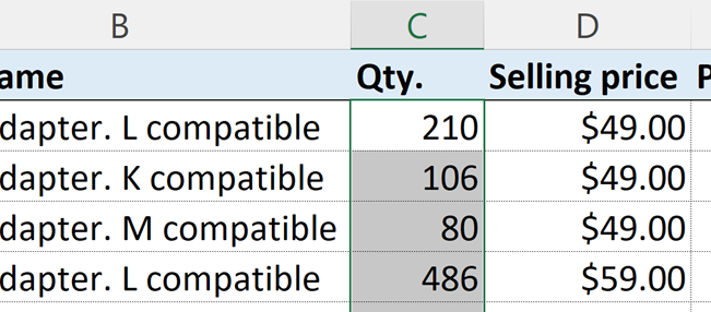
With those selected cells, we need to apply a ‘Highlight Cells’ conditional formatting rule.

2. In the Home tab of the ribbon, click ‘Conditional Formatting’.

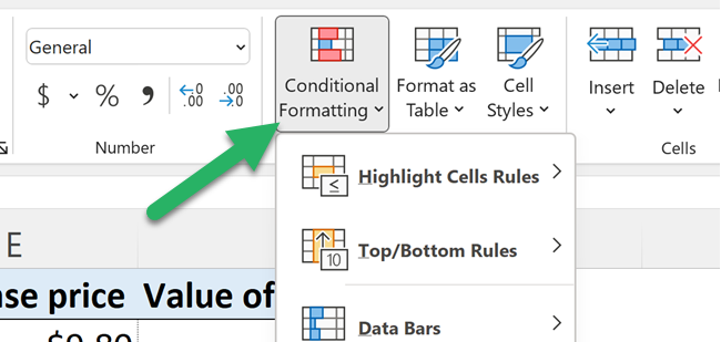
3. Hold your cursor over ‘Highlight Cells Rules’ and click ‘Less than’.

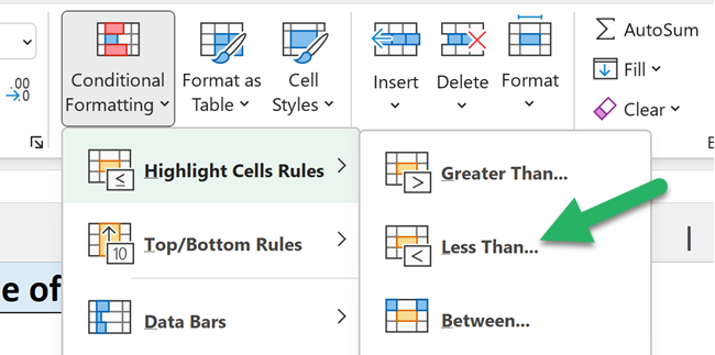
This conditional formatting rule allows you to apply conditional formatting if the value of a cell is less than what you’re defining in a few seconds.

4. In the left field, write the number the cell value should be less than to apply conditional formatting.

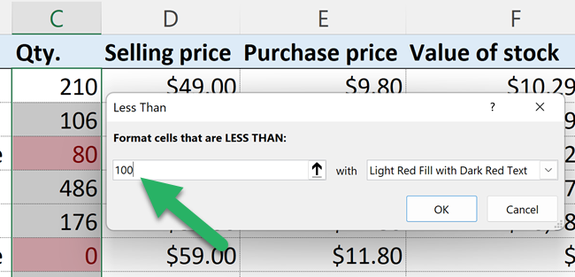
As you type, you can see the format of this conditional formatting rule being applied to the selected cells.

Right now, it’s just the standard format: Light Red Fill with Dark Red Text.

Classic👍

5. In the right field, click the drop-down button if you want to change to another formatting preset.

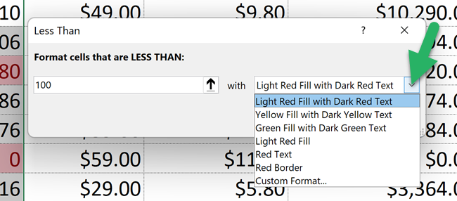
6. Or you can click ‘Custom Format’ to control the formatting style 100%.

And that’s it.

Watch all the values below 100 being highlighted automatically. Beautiful, isn’t it?💕

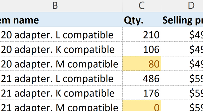
This conditional formatting rule can be modified to other situations if you take a step back.

For instance, you can turn it upside down and highlight cells that are above 100.

Or cells with values between 50 and 150.

The possibilities are almost endless.

Highlighting entire rows based on a formula

Entire rows look nice when they are formatted in a certain way. Instead of random colored cells everywhere.

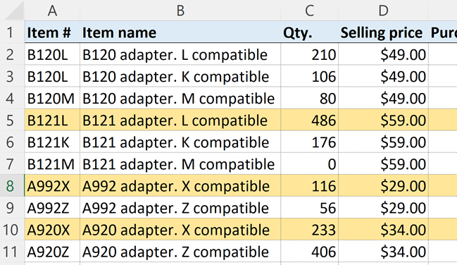
So, let me show you how to color an entire row with a conditional formatting rule if the value in column C is less than 100👀

1. Select the entire data set. The selected cells indicate how much of each row is highlighted by the conditional formatting rule.

2. Click ‘Conditional Formatting’ on the Home tab and click ‘New Rule.’

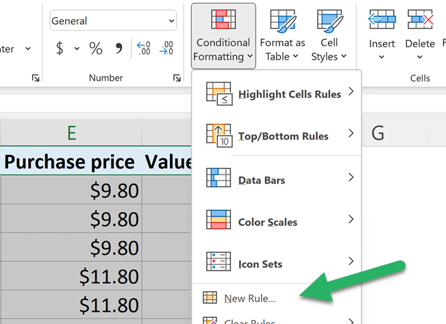
3. In the dialog box that appears, select ‘Use a formula to determine which cells to format’ from the ‘Rule Type’ menu.

4. Right below, enter this formula:

=$C1<100

So, if the value in column C drops below 100, the conditional formatting rule triggers.

You can’t refer to entire columns, so you need to refer to C1. NOT C2, although it seems more logical⚙️

If your data starts in row 3, 5, 10, or whatever other row, the reference still goes to C1 (or whatever column you’re using).

5. Now chose your formatting style from the ‘Custom Format’ button.

Or settle for the standard preset.

And behold!

All the cells in your data rows are now formatted, and not just in 1 column like they typically are with conditional formatting.

Editing and removing conditional formatting rules

The layout and use of a workbook are rarely static, so the conditional formatting that you apply to your sheet may have to be edited at some point.

For instance, the previous highlight cells rules we set… Maybe it’s time to change them.

Luckily that’s fairly easy.

You can edit any conditional formatting rule from the conditional formatting rules manager.

Edit the conditional formatting rule and formatting style

1. Click ‘Conditional Formatting’ from the Home tab and select ‘Manage Rules’.

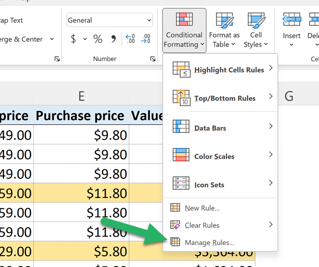
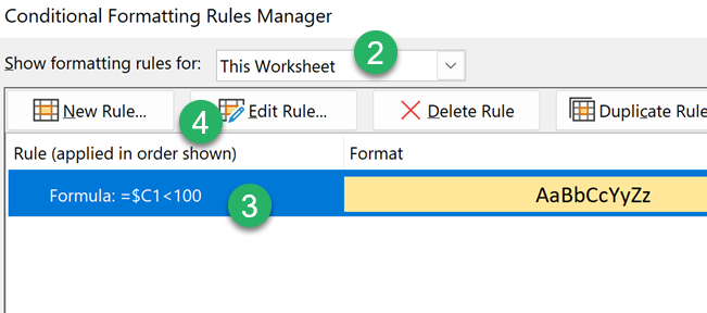
After you click ‘Manage Rules…’ you’ll see a ‘Conditional Formatting Rules Manager’ dialog box.

Change the following 3 points as you see them on in the manager.

2. Set ‘Show formatting rules for:’ to ‘This Worksheet’ to show all conditional formatting rules for the entire sheet.

3. Find the rule you want to edit (there might be several on the list).

4. Click the ‘Edit Rule’ button.

Another dialog box appears. From here you can change anything about the rule.

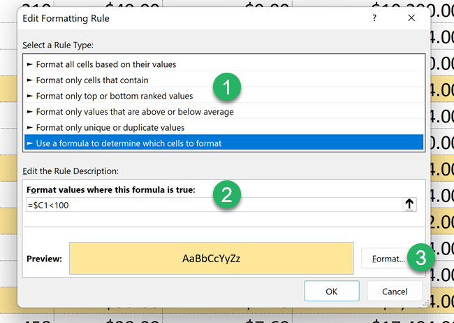
Below we’ll go through the different options shown in the screenshot above.

Circle 1) Here you can change the ‘Rule Type’. If you don’t want to apply conditional formatting when “something” happens in a cell, you can change it to apply on all cells and fill them with color based on their value compared to the average of the data.

Circle 2) If you keep the ‘Rule Type’ you can change the “trigger” of the formatting. The trigger depends entirely on which type of conditional formatting rule you choose in circle 1. In this case, you can change the custom formula.

Circle 3) From this little (familiar) box you can change the formatting that you applied in the first place. If you don’t want your cells to turn yellow when it drops below cell value: 100, you can have them turn purple instead.

As you see there are more than enough options.

But wait – there’s more!

Edit the conditional formatting rules range

All of the above is very nice, but if you accidentally selected the wrong area when you made the conditional formatting rule – then it doesn’t help to change the ‘Rule Type’ or whether the cells should be red or blue.

And if you spent 5 minutes entering a unique formula to “trigger” the formatting, then it sucks to delete it and do it all over.

To change the range of cells that the conditional formatting applies to, you don’t need to go to the ‘Edit Rule’ box above.

You just need to click in the ‘Applies to’ column at the rule you want to change in the ‘Conditional Formatting Rules Manager’ box.

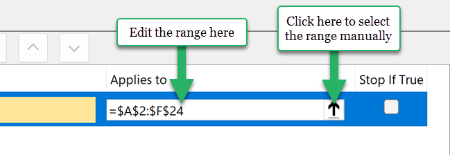
If you can’t remember the range that the rule should apply to, click the tiny red arrow to select the range manually.

That’s how you edit a conditional formatting rule✏️

So if you screw one up?

You don’t have to delete it – simply just edit it.

Delete a conditional formatting rule

Sometimes you see a workbook with too many conditional formatting rules.

This can create immense confusion and on top of that, it can make your workbook slow.

In this case, you need to remove conditional formatting from the spreadsheet. Maybe even all of it!

Click the ‘Conditional Formatting’ button on the ‘Home’ tab and hover your mouse over ‘Clear Rules’.

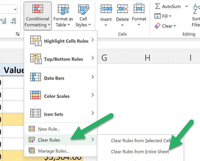
Then click ‘Clear Rules from Entire Sheet’.

That was pretty easy. But it’s not always clever to clear all conditional formatting rules from a sheet!

Sometimes some rules should still apply.

To select specifically which conditional formatting rules are to be removed, click ‘Manage Rules…’ instead.

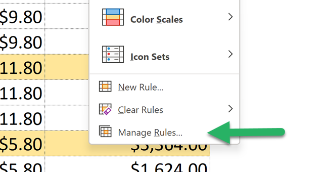
Here you’ll find the conditional formatting rules manager dialog box that you can use to clear rules, in addition to editing rules.

To delete specific conditional formatting rules:

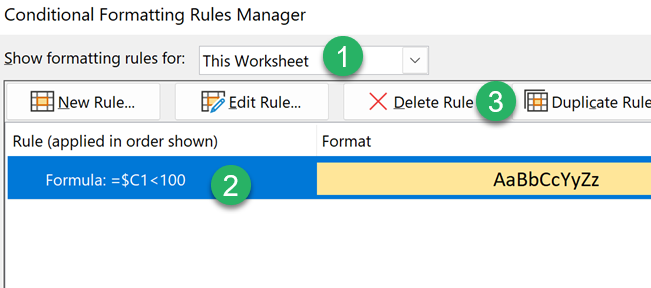
1. Click the drop-down arrow that initially says “Current Selection”. Change it to “This Worksheet”.
2. Select the conditional formatting rule you don’t want anymore.
3. Press ‘Delete Rule’ to actually clear rules.

Remember to click OK when you’re done.

And that’s how you actually clear rules✏️

That’s it – Now what?

That’s how to highlight cells with conditional formatting.

Like all the cells that contain a specific word or a number.

Heck, you even learned how to remove conditional formatting, create a new rule from a formula, and much more.

Well done💪

Conditional formatting is a part of Excel that can think for itself. Meaning it makes its own decisions. It “reads” the cell and reacts on the content.

There are several other parts of Excel that react to the content of cells – just like conditional formatting does.

And you most definitely want to learn those parts.

So, I’ve made a free course teaching you 2 of the best conditional functions Excel has to offer: IF and SUMIF.

Also, you learn VLOOKUP and pivot tables.

Click here to enroll in my free 30-minute course and I’ll send it to your inbox right away.

Other resources

There are several other ways of using conditional formatting.

Instead of highlighting specific cells, you can visualize high/low values in an entire data set in a few seconds with data bars, icon sets, and color scales.

Another cool feature of conditional formatting is that you can highlight duplicate values.

Or you can use this neat conditional formatting tricks to highlight every other row.

Oh, and here’s the best way to remove normal formatting, in case you want to apply new formatting.

Frequently Asked Questions

If you’re looking for a specific answer to a specific question, please see the FAQ section below. Maybe you’ll find what you need😊