How to use INDEX MATCH
with Multiple Criteria in Excel

INDEX MATCH with multiple criteria enables you to look up and return values even if there are no unique values to look for.

This is not achievable with any other lookup formula without inserting helper columns.

In this guide, you learn the three steps to make it work every time😊

Grab the workbook here so you can tag along, and let’s set the scene with an example below.

Example of using INDEX MATCH with Multiple Criteria

So, you got this employee database.

You want to make the database easier to search, so you’re creating a small tool (to the right in the worksheet).

In that tool, anyone should be able to type in the name and division of an employee and it will find that person’s salary (and show it in cell G4).

“That’s easy, I can just use VLOOKUP.”

Wait a minute✋

Unfortunately, it’s not that easy.

You see, the problem is that there are actually two employees called “Steve Jones”. That means the lookup value has two matches in the lookup column (column a).

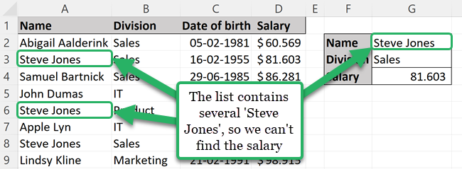
There’s nothing unique about Steve Jones’ name on its own.

In Microsoft Excel terminology, ‘Name’ would be one criterion.

So, one criterion didn’t cut it.

But if you include another criterion, like ‘Division’, you make Steve Jones unique.

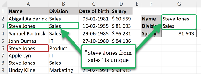
Now, while “Steve Jones” appears several times on the list, there’s only one “Steve Jones from the sales division”.

This is the kind of magic you can do with INDEX MATCH with multiple criteria.

Now, follow the 3 steps below to learn how this wonderful formula works 😊

Step 1: Insert a normal INDEX MATCH formula

INDEX MATCH with multiple criteria is an array formula created from the INDEX and MATCH functions.

The synergies between the INDEX and MATCH functions are that:

• MATCH searches for a value and returns a location
• MATCH feeds the location to the INDEX function
• Then INDEX transforms this location into a result

Start the formula

First, start the MATCH function, and then put the INDEX function around the MATCH function to complete the formula.

Start with:

Step 1.1) As the first argument in the MATCH function, enter the lookup_value. This is what you are looking for.

In this case, you’re looking for an employee with the name “Steve Jones”.

Select (or manually enter) cell G2 as the lookup_value, then separate with a comma to move on to the lookup_array.

Step 1.2) The lookup_array is the column where the MATCH function looks for the lookup value.

Select the column with the names, and then enter a comma to move on to the [match_type].

Now your formula should look like this:

Step 1.3) A little drop-down list appears that gives you the choice between 1, 0, and -1.

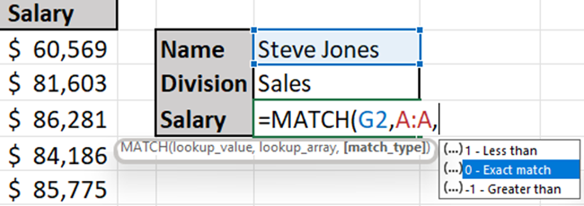
The 0 option is the Exact match option and is most commonly used.

The -1 and 1 are similar to VLOOKUP’s “approximate match” method.

Write 0 or double-click the 0 – Exact match option in the drop-down menu and type the end parenthesis.

Your formula should now look like this:

Step 1.4) Wrap the INDEX function around the MATCH function.

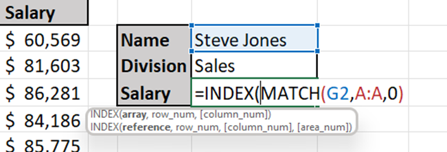
Your formula should look like this by now:

But we’re not done yet✋

The syntax of the INDEX function goes:

INDEX(array, row_num, [column num])

The MATCH function should be the second argument in the INDEX syntax.

Right now, it’s the first argument.

So, begin writing the real first argument: the array.

The INDEX array is the column you want to return values from.

The purpose of the multiple criteria INDEX MATCH is to find the salary of a specific employee.

So, the array is the salary column (column D).

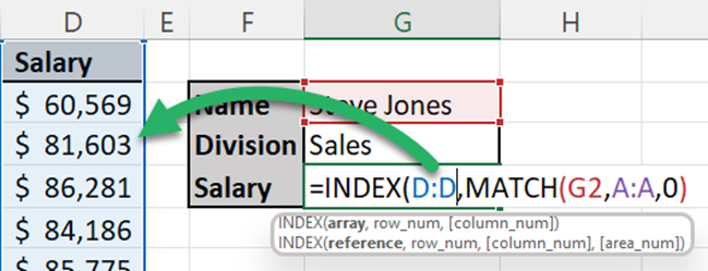
Your formula should look like this by now:

Just put an extra parenthesis at the end to wrap up the INDEX function.

So, the final formula looks like this:

EXPLANATION

The MATCH function searches for the value in G2 (“Steve Jones”) in the database and then returns a number.

This number is the row in the dataset where the name “Steve Jones” is found.

This row number is then fed into the syntax of the INDEX function.

Step 2: Change the lookup value to 1

Now, you need to change your normal INDEX MATCH formula into an array formula.

Sounds hard?

Don’t worry, I’ll guide you step-by-step😊

Step 2.1) Change the lookup_value of the MATCH function to 1.

So, the formula changes from:

To:

The “theory” behind this is not as simple as changing the lookup_value.

Since you’re changing the formula from a normal one to an array formula, the structure of the formula changes a bit as well.

By changing the lookup_value to 1, you’re not actually telling the MATCH function to search for the number 1 in the lookup_array (name column).

When you enter our two criteria in the next step, the 1 in the MATCH function simply means:

“Look through the rows in the data and return the row number where all of the criteria are TRUE”.

If you wrote a zero, the formula would look for a row where all of our criteria are FALSE – and that wouldn’t really make sense.

Step 3: Write the criteria

The criteria replace the second argument of the MATCH function, with this structure:

(range=criterion1)*(range=criterion2)*(range=criterion3)*…

This way, you can have as many criteria as you need.

INDEX MATCH function with two criteria

It’s typically enough to use two criteria to make your lookup value unique.

Criterion 1 = name

Criterion 2 = division

Let’s see if you can find “Steve Jones from sales” or if he’s lost in the woods🌳

Step 3.1) Replace this structure: 

(range=criterion1)*(range=criterion2)

With the actual criteria:

(A:A=G2)*(B:B=G3)

• A:A is the column with names.
• G2 is the name you’re looking for.
• B:B is the column with division.
• G3 is the division you’re looking for.

Step 3.2) Write that as the second argument in the MATCH function, replacing what’s currently there.

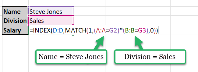
Your INDEX MATCH formula should now look like this:

If you want to go with 3 criteria, you add the 3rd criterion to the criteria structure:

(range=criterion1)*(range=criterion2)*(range=criterion3)

Converted to actual ranges and criteria, it would look like this:

(A:A=G2)*(B:B=G3)*(C:C=G4)

Step 3.3) If you’re using Microsoft 365 just press Enter and watch your beautiful multiple criteria lookup💡

If you’re not using Microsoft 365, do not press Enter when you’re done with the formula. It won’t work. Instead, press Ctrl + Shift + Enter.

Explanation: Ctrl + Shift + Enter

If you don’t have Microsoft 365, array formulas need to be handled differently than other formulas.

So, instead of pressing Enter, press Ctrl + Shift + Enter when you are done with the formula.

Warning: {curly brackets} will appear around your formula. They are supposed to be there!

Every time you make changes to this formula, you must end with Ctrl + Shift + Enter

(Instead of just regular “Enter” as you are probably used to)

Conclusion

Wow… You just learned how to use INDEX MATCH with multiple criteria…

It wasn’t so scary after all, right? 😎

Now, you’ve created a tool to easily look up employees and return their salary – even if there are multiple employees with the exact same name!

All are fueled by the INDEX and MATCH functions.

You may also be interested in

My brand-new video on INDEX MATCH with Multiple Criteria (make sure to like and subscribe!)

Excel INDEX MATCH is not the only lookup formula out there (although it’s the only one you can turn into an array function).

If you want to expand your toolbox further, definitely get to know the VLOOKUP function, HLOOKUP, and the new XLOOKUP.

If you thought this guide was hard to follow, you should dive into the INDEX and the MATCH functions separately.

Besides, there’s another, underrated, way to achieve a lookup with multiple criteria. That’s the good old Excel filter.

Finally, you might also enjoy my pivot table tutorial or my favorite collection of project management templates.