How to Use Excel’s Annuity Formula (Easy Example)
The word of annuity might be one of the unheard or less-heard ones for you but believe me, we see the concept of annuity practically applied almost everywhere around us.
Most of the financial products you’ve arranged with your bank or provider are annuity arrangements. Surprised? 😲
What is an annuity? How is it applied in the real world? How do you calculate it in Microsoft Excel?
Get answers to all these questions boggling in your head in the tutorial below. Grab your free practice workbook for this guide here, and come along with me.
What is Annuity
An annuity is a financial arrangement that’s set to make a series of cashflows at predetermined time intervals in the future.
Annuities are mostly contracts set up by insurance companies to offer a steady cash flow to people who have reached their retirement 🧓
A very simple example of an annuity is that you’re reaching your retirement in a few years so you start searching for good retirement packages that can take care of your post-retirement life.
And let’s you come down to one of the most suitable packages for yourself that says
- if you deposit $125,000 (lump sum) to the insurance company by the date of your retirement,
- you get $12,000 each year for 25 years post-retirement
This is an annuity contract where you’re paid a series of cashflow ($12,000 each year) on pre-determined regular intervals (each year-end for the coming 25 years) 📆
Formula of Annuity
Annuity discounts or compounds a given set of cash flows based on the period when they occur.
Present Value of Annuity
The present value of annuity discounts cashflows occurring in the future at a certain discount rate to calculate their today’s value.
If the cashflows are not the same, for example you get $100 in Year 1, $200 in Year 2, $250 in Year and so on, discount each cashflow separately and sum them up.
Whereas, if the cashflows occurring in all future years are identical, say $100 each year for the coming 10 years, the above formula can be concise as:
- CF = Cashflow
- I = Periodic Interest rate
- N = Number of annuity payments period
Future Value of Annuity
The future value of an annuity calculates the value of a series of cash flows occurring at certain intervals at a certain date in the future (mostly the date when the payment intervals end).
For example, if you’re getting $100 for 5 years each, what would be the total value of all these cashflows at the end of year 5? 🤔
How to calculate annuity in Excel
Let’s now see how you can calculate annuity in Excel.
Depending on whether you want to calculate the PV of annuity or FV of annuity, we have different functions in Excel that enable you to calculate them both.
Present value of annuity (PV function)
Let’s continue with the same above example. So, let’s say you’re retiring in 2035. Your insurance company has given you the following package.
- Deposit $125,000 with us by the end of 2035
- You’ll receive a guaranteed cash payment of $12,000 for 25 years starting from 2036
- The interest rate fixed in this contract is 10%
Before you sign up for this contract, do some math to see if it is even worth it to invest this much money with them💸
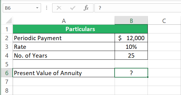
To do so, we will calculate the Present value of this annuity by using the PV function of Excel.
Step 1) Begin writing the PV function as below:
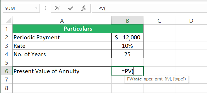
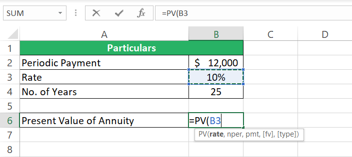
Step 2) For the rate argument, refer to the interest rate.
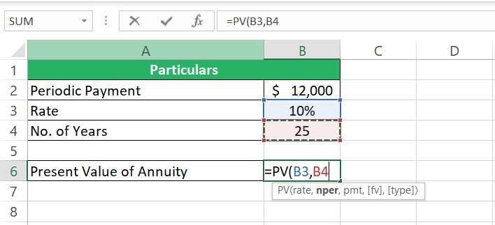
Step 3) For the nper argument, refer to the number of periods i.e., 25 years.
Step 4) The pmt argument refers to the equal cashflows to occur each year so we’re referring to Cell B2 ($12,000) as pmt.
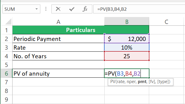
Step 5) The pv argument refers to the present value of cash flows. It is optional but must be given if you omit the pmt argument.
Since we are finding the PV for these cashflows and have supplied the value for pmt, we will omit it.
Step 6) The type argument is also optional. Omitting it sets it to 0, which means the cash flows occur at each year’s end.
Alternatively, you can set it to 1 if the cashflows occur at the period beginning instead of year-end.
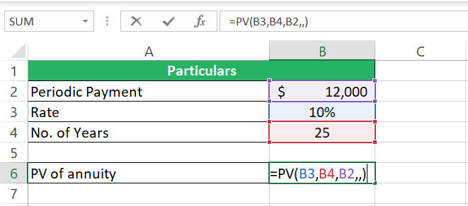
Step 7) Hit Enter to have the PV of your annuity calculated.
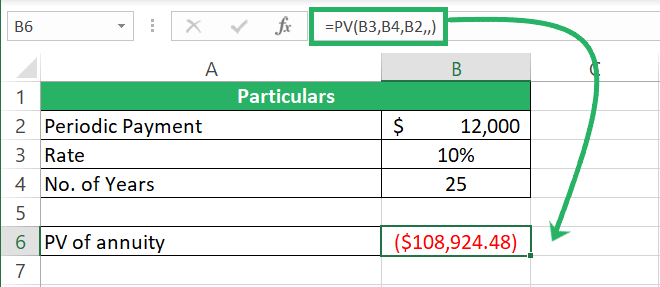
Excel returns the PV of this annuity as $108,924.
The PV appears as a negative number since Excel understands it is a cash outflow. This should be the amount deposited to the insurance company to receive $12,000 cashflows in the future years.
Besides your decision if you want to invest in this annuity or not, are you curious as to how Excel calculated $108,924 and if it is even correct?
Let me show you the math run by Excel to reach this value.
Step 1) Discount each year’s cash flow by using the following annuity formula.
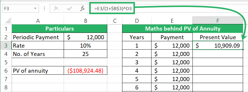
Step 2) Drag and drop the formula to the whole series of 25 years.
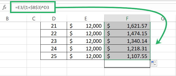
Since we have identical cashflows of $12,000 occurring over all the 25 years, you can also use the concise formula discussed in the first section. I discounted each cash flow individually just to paint the complete picture before you.
Step 3) Now sum all the discounted cashflows up to reach the total present value of the annuity.
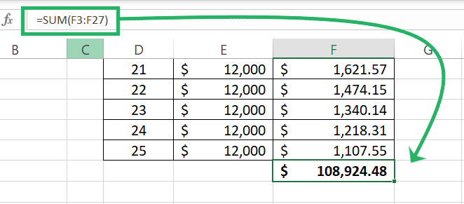
The numbers match 🤩
This is what Excel’s PV function does for you.
Periodic payments of annuity (PMT function)
Another annuity-based function of Excel is the PMT function.
It helps you find the yearly constant payments to be made assuming a constant interest rate to reach a certain future or present value of the annuity 😎
To understand the PMT function, let’s assume you’ve signed up for the above contract.
This means you have to deposit $125,000 in your insurance bank account by 31 December 2035. Assume, it’s 01 January 2024 today.
You have 12 years starting from now to pool up that amount 📃
It’s not easy to deposit a lump sum amount of $125,000 so why don’t you start salting away some money early for the coming 12 years?
If your bank pays 10% annual interest on your deposits, how much money should you pay each year to have a lump sum of $125,000 ready in your account after 12 years?
Let’s find it out using the Excel PMT function.
Step 1) Begin writing the PMT function as below:
Step 2) For the rate argument, refer to the interest rate.
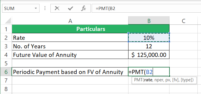
Step 3) For the nper argument, refer to the number of periods i.e., 12 years.
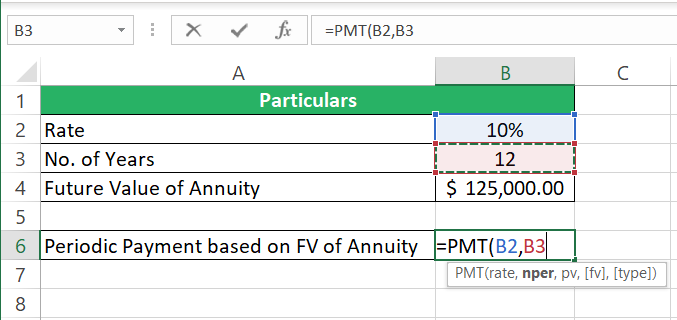
Step 4) Omit the pv argument since we do not know it.
Step 5) The fv argument refers to the future value of the cash flows. We want the future value of these cashflows to be $125,000. Refer to the same as the fv argument.
Step 6) Omit the type argument so that it defaults to 0 since we will make the payments at year-end.
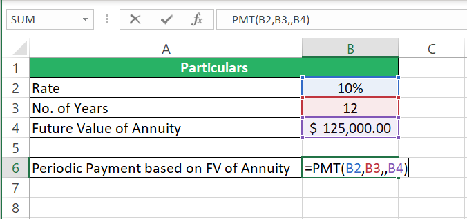
Step 7) All done. Press Enter.
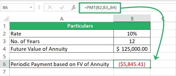
There you have it. Deposit $5485 in your account each year for 12 years and you’d have $125,000 compounded in your account by Year 12 💰
This time Excel has returned the annual PMT as a negative value because we supplied the FV as a positive value. Accordingly, Excel understands that the annual payments will be cash outflows.
Reassurances are never bad, are they?
Let’s run a quick background math to check if 12 annual compounded deposits of $5485 will grow to $125,000 by Year 12 🔎
Step 1) Compound each year’s cash flow by using the following annuity formula.
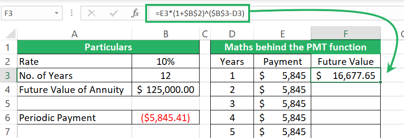
You make the first deposit of $5485 in your account at the end of 1st year i.e., 31 December 2024. It stays in your account for only 11 years. This is why I have deducted the year of deposit (1) from the number of compounding years (12).
Step 2) Drag and drop the formula to the whole series of 12 years.
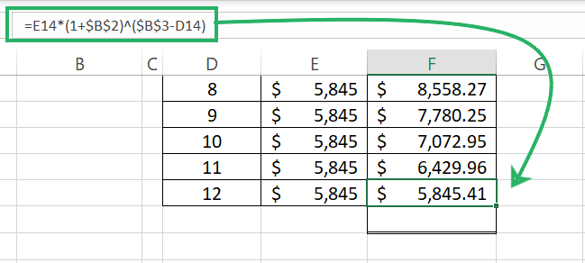
Step 3) Sum all the compounded cashflows up to reach the total future value of the annuity.
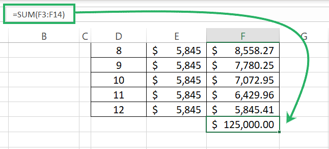
What a precise match. You’ll have exactly $125,000 in your account by Year 12.
Future value of annuity (FV function)
The future value of the annuity is the opposite concept of the present value of the annuity.
Here’s a quick example for you to understand this.
You sign a contract with your insurance company to 📝
- Pay them $12,000 each year (at year-end) for 12 years
- And at the end of 25 years, they will pay you a lump sum of $250,000
- The interest rate for this agreement is 10%
How can you check if you’re paid the right amount (of $250,000) by the end of your retirement package?
You can calculate the FV of your annuity by using the FV function of Excel. Check here.
Step 1) Begin writing the FV function as below:
Step 2) For the rate argument, refer to the interest rate.
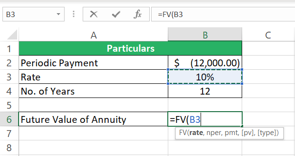
Step 3) For the nper argument, refer to the number of years.
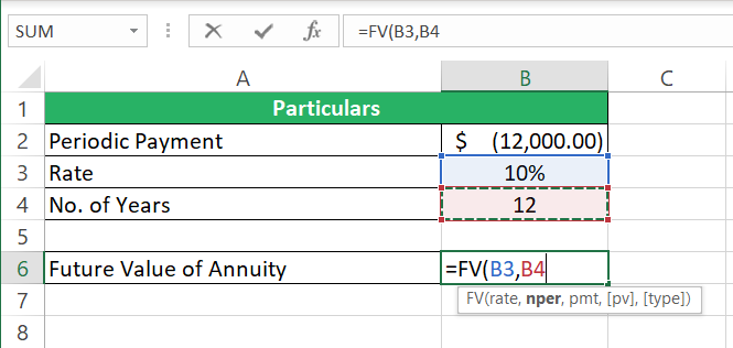
Step 4) For the nper argument, refer to the periodic payments to be made.
Step 5) Omit the pv and type argument.
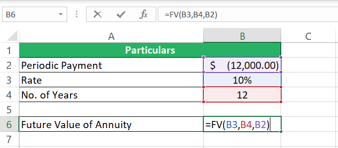
Step 6) And hit Enter.
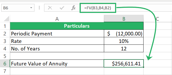
Excel returns the FV of this annuity as $256,611.41.
Here’s how Excel calculated it.
Step 1) Discount each year’s cash flow by using the following annuity formula.

Step 2) Drag and drop the formula to 12 years.
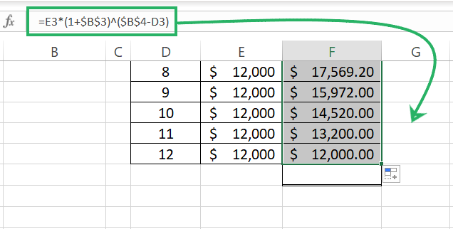
Step 3) Sum up the compounded cashflows.
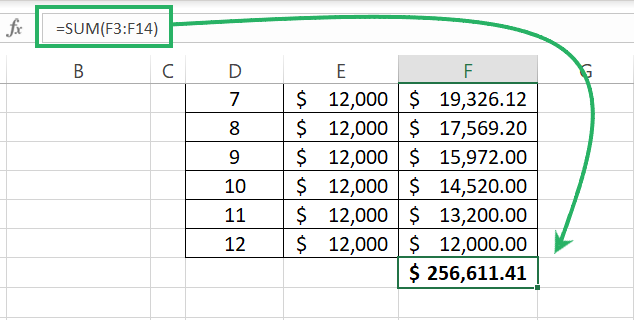
This tells that if you keep depositing $12,000 each year for 12 years compounded at a 10% interest rate, you’d have a balance of $256,611 by the 12th year-end 🚀
Annuity Vs. Annuity Due
While you calculate annuity in Excel, be mindful of two different types of annuities:
- Annuity: Under the normal annuity, periodic payments are made at each period’s end.
- Annuity Due: Under annuity due, the periodic payments are made at the beginning of each period.
This makes quite some difference to your annuity calculation and the result since the time when a payment is made determines the period for which it should be discounted or compounded ⌛
For example, if the payments for the following insurance agreement are made at year-end (ordinary annuity), the present value of the annuity would be.
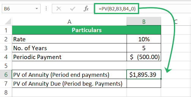
Whereas, if the payments for the following insurance agreement are made at the beginning of the period (annuity due), the present value of the annuity would be
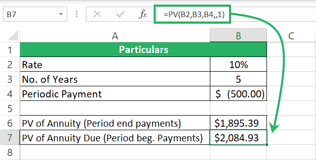
Setting up both the annuity types in Excel is super easy:
- For Annuity (period-end payments), set the type argument to 0 or omit it.
- For Annuity due (Period beginning payments), set the type argument to 1
Conclusion
Annuity is a very interesting concept of corporate finance. What I find even more interesting about annuity is the calculation of annuity.
It is exciting to calculate the present value, future value, and periodic payments for different annuity packages (only if you understand the science of what runs behind the annuity formula). However, if you’re running short on time, ditch the manual formulas and use the smart PV, FV, and PMT functions of Excel explained above.
If you enjoyed reading this tutorial, you’d enjoy the following my Excel tutorials on the following financial functions / topics, too. Give them a read.
