Cell References in Excel: Relative, Absolute, and Mixed
Cell references often confuse Excel users no matter how simple they may sound.
Be it Cell A1 or Cell XFD1048576. How are these cell references made?🤔
The guide below will teach you this and much more. So jump right in.
And as you go, download our free sample workbook here to practice along the guide.
Table of Contents
What are cell references in Excel
Cell references are like the name of cells. A cell reference is alphanumeric; it consists of an alphabet and a number. 🔠
Where do this alphabet and number come from? Here is what a worksheet in Excel looks like (A two-dimensional window with rows and columns).
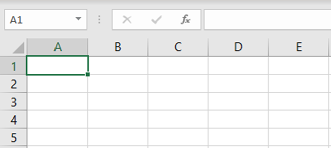
Columns in Excel are denoted by alphabet. Whereas rows in Excel are denoted by numbers.
A cell is formed at the intersection of a row and a column. It is then named as a combination of that row and column.
For example, in the image below the highlighted cell forms at the intersection of Column B and Row 2.
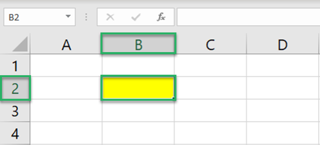
The highlighted cell is referred to as Cell B2 (Column B and row 2).
Similarly, drag your worksheet to the end to see if even the last cell (Cell XFD1048576) is referred to the same way.
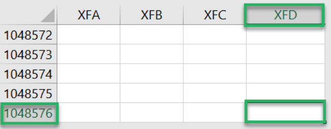
It is formed at the intersection of Column XFD and Row 1048576.
Pro Tip!
Did you know? There are a total of 16,384 columns in Excel. And the total number of rows in Excel is 1,048,576. 💯
How to use cell references (relative references)
Cell references make your Excel jobs unbelievably easy. You can use them everywhere and the best thing – as you move the formulas, the cell reference automatically adjusts.
See here.

The image shows the total marks for each subject in Row 2. The percentage marks acquired by a student in each of these subjects is in Row 3.
Let’s quickly find the marks scored in each subject.
Write the formula in Cell B4 as follows:
= B2 * B3

We are multiplying Cell B2 (Total marks) by Cell B3 (Percentage). Excel calculates the obtained marks in English.

Let’s calculate the same for the remaining subjects. But don’t waste time writing the respective formula for each subject.
Drag and drop the formula in Cell B4 to the remaining cells.

Excel calculates the obtained marks for all the remaining subjects.
But what has Excel done?
When formulas are moved across cells, Excel changes the relative cell references based on the relative rows/columns.
For example, the above formula when copied from Column B to C becomes:
= C2 * C3

Move it from Column C to Column D to see it changes as follows.
= D2 * D3

That way, you do not have to write formulas unique to each cell.
You can put together a single formula for one cell and copy/paste it to the others. Excel will automatically update the relative cell references. 💪
How to use absolute cell references
What if the above data changes as shown below?

The data remains the same. However, marks for each of the subjects are not mentioned now. Instead, we have the total marks in Cell F2 only.
To calculate the marks obtained in English, write the formula below.
= B2 * F2

B2 consists of the percentage marks obtained in English. At the same time, Cell F2 consists of the total marks for all the subjects.
Excel calculates the marks obtained in English as below.

Can we move the same formula (drag and drop it) for the remaining subjects?

The results are bizarre. What has Excel done?

The cell references were relative. As we moved it from one column to another, Excel changed the column reference from F2 to G2. G2 is an empty cell, so, Excel returns zero.
In such a case, we don’t want Excel to change the cell reference (F2) every time the formula is moved. We want to keep it constant.
However, we want the cell reference for percentages to change every time the formula is moved.
Write the formula as follows.
= B2 * $F$2

We have changed the relative reference of Cell F2 into an absolute reference of $F$2.
Unlike relative cell references, an absolute cell reference has a dollar symbol before the column and the row reference. Like $A$1.
However, the cell reference B2 is still the same. This is because we only want to fix the cell reference $F$2 but not B2.
Drag and move it across all the columns

Excel calculates the obtained marks for all the subjects.
This time Excel updated the formula for each next column by changing the cell reference of B2 but not F2.
For example, when moved to Column C, Excel changes the formula as below.

So, the formula changes from:
=INDEX(D:D,MATCH(G2,A:A,0))
To:
=INDEX(D:D,MATCH(1,A:A,0))
The “theory” behind this is not as simple as changing the lookup value.
Since you’re changing the formula from a normal one to an array formula, the structure of the formula changes a bit as well. By changing the lookup value to 1, you’re not actually telling the MATCH function to search for the number 1 in the lookup array (last name column).
Pro Tip!
To change any reference into an absolute cell reference, click on that cell reference in the formula bar and press the F4 key.
Mixed cell referencing in Excel
Who said a cell reference has to be a relative or an absolute one only? There can be mixed cell references too.
Pro Tip!
A mixed cell reference is where any one component of the cell reference (column reference or the row reference) is absolute, and the other is relative.
For example, $C3 (Absolute column reference and relative row reference). Or C$3 (Relative column reference and absolute row reference).
The absolute reference comes after a dollar sign. 💲
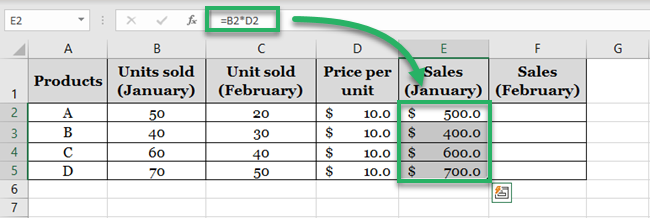
For example, the image below the number of units sold for January and February.
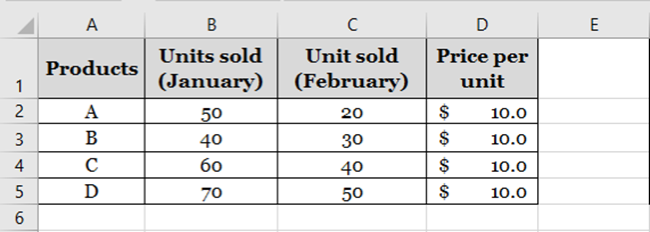
To calculate the sales for both months, let’s multiply these by the price.
- Write the formula as:
= B2 * D2

- Drag and drop the same formula to all the products to get the sales for January.
What about February?
- Copy-paste the same formula into the column for February sales.
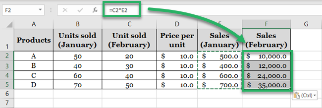
This is what happens when you do so. As we move the formula one column ahead, Excel changes the column references from B2 and D2 to C2 and E2.

We want Excel to multiply the units sold of each product for each month with the price. This means we want to keep the column of prices (Column D) constant.
- To do so, convert it into a mixed reference as follows.
= C2 * $D2

We only added a dollar sign ($) before the column reference (D). There is no dollar sign ($) before the row reference (2).
This way each time this formula is moved, the column will remain the same (Column D), but the row number would accordingly change.
- Drag and drop the formula now to see the results.

Excel now keeps Column D constant. All other references change with the relative position of the row/column.
Cell references to other worksheets
Cell references are not limited to a single sheet only. You can also create a reference to a cell from another worksheet. 🙌
See here. We have the value for Apples in Sheet 2.
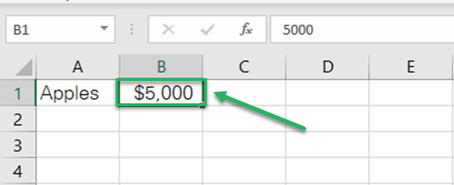
We need this sales value in Sheet 1.
- To create a direct reference to Sheet 2, activate a cell in Sheet 1 and write an equal sign (=).
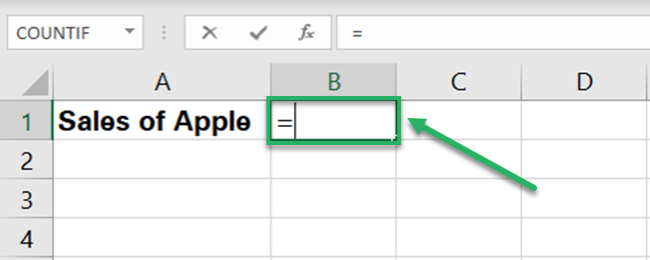
- Now go to sheet 2 and click on the targeted value (sales value of Apples).
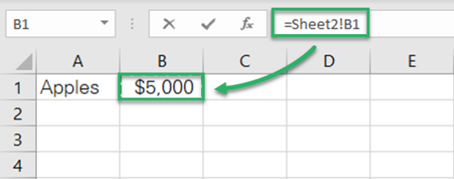
- Press Enter.
- In sheet 1, a reference is created to Cell A2 of Sheet 2.
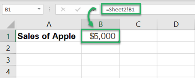
That is how you can create references to other cells across different worksheets of a workbook.
That’s it – Now what?
Cell references are one of the building blocks of Excel. Unless you understand how cell references work, you can barely use Microsoft Excel.
👉 The above guide teaches you how cell references are formed. We learned about all three types of cell references (mixed, relative, and absolute references). And also how they can be used within a worksheet and across worksheets.
To make your Excel jobs even simpler, you must master the SUMIF, IF, and VLOOKUP functions of Excel.
Click here to sign up for my 30-minute free email course that teaches you these and other functions of Excel.
Other resources
If you enjoyed learning about cell references, we bet you’d love to know more.
Just like cell references, there’s so much more to the basics of Excel that will change the way you work. Hop on here to learn how to select multiple cells and merge/unmerge cells in Excel.
