How to COUNTIF Between Two Numbers in Excel: Step-by-Step
Looking for a simple way to count the number of cells in Excel that fall within a specific range of values?
Look no further than the COUNTIF function!
In this tutorial, we’ll show you how to use this powerful tool to count cells between two numbers in just a few clicks.
So whether you’re an Excel pro or just getting started, read on to learn how to make the most of this function 💪
You can download our sample workbook here to practice the COUNTIF function in real time.
Count if between two numbers
COUNTIF can be very helpful in counting numbers that meet specific criteria. But similar to COUNTIF, there is another function COUNTIFS.
Although both these functions are used to count numbers, there is an important difference between them 🤔
COUNTIF is used to count cells that meet a single condition. For instance, you can use COUNTIF to count cells containing the number 10 or numbers less than 50.
Its syntax is:
=COUNTIF(range, criteria)
The COUNTIFS function is used to count cells that meet multiple criteria. For example, you can use the COUNTIF function to count cells that contain the number 10 and are less than 50.
Its syntax is:
=COUNTIFS(criteria_range1, criteria1, [criteria_range2, criteria2], …)
In short, both serve the same purpose but on a different scale.
In this guide, we will be focusing on how COUNTIF can help count numbers between two values. Let’s see how to do it below.
Say, we have the following sample data.
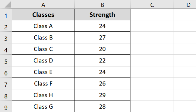
It contains information about the number of students in different classes.
We want to count the number of classes that have strength between 20 to 25. We will use the COUNTIF function for this purpose 😀
To do this,
- Select a blank cell.
- Type in the COUNTIF formula as:
=COUNTIF(
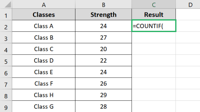
- Enter the data range containing the strengths of the classes.
=COUNTIF(B2:B10,
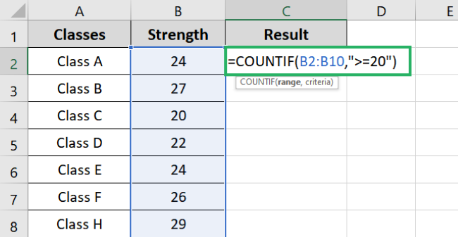
- Enter the criteria or condition you want to apply. It can be a number, text, reference, etc.
=COUNTIF(B2:B10, “<20”)
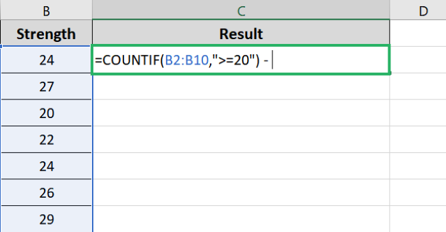
Note that your condition should be accurate.
If you want to count classes having a strength of 20 and less, then the condition will be “<=20”. But if you only want to count classes having a strength less than 20, set the condition as “<20”.
Make sure to add double quotes before the criteria.
If you’re thinking we’re done here – you’re wrong. There is another step before we get our final result 🤓
- Add a minus sign after closing the bracket.
- Type in the formula again as:
=COUNTIF(
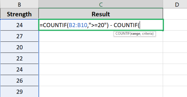
- Add the data range.
=COUNTIF(B2:B10
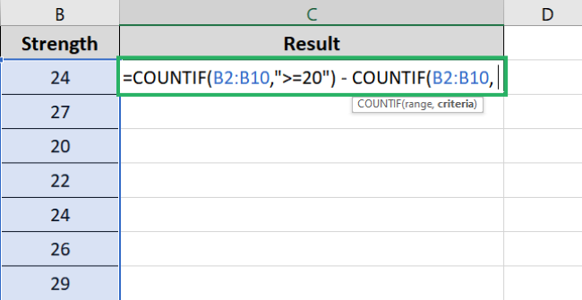
- Add the second condition to the formula.
=COUNTIF(B2:B10, “<25”)
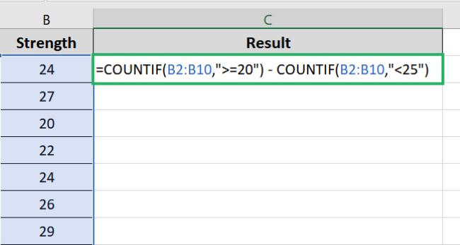
- Press Enter.
Excel will return the result as:
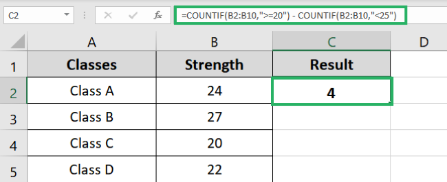
As evident, the formula returns 4, which is the number of classes whose strength lies between 20 and 25.
Pretty easy, no? Try it yourself using the sample workbook provided 🧐
That’s it – Now what?
In this article, we saw how to use the COUNTIF function to count cell numbers. The function does most of the work, and you can get the remaining help from this guide.
The COUNTIF function is a statistical function that counts cells based on criteria. For instance, you can use COUNTIF to find how many times a particular value occurs in the sheet.
It is used for a variety of purposes. Luckily, Excel has a plethora of functions that are just as fantastic as COUNTIF 😎
Our favorite Excel functions include SUM, SUMIF and VLOOKUP. You can learn them for free in my 30-minute free email course only at the cost of your email address. So sign up now!
Other resources
Do you enjoy reading this article? If yes, then we’re sure you’d love to read more.
Try similar topics: COUNT, COUNTIF, Greater than with SUMIF and COUNTIF and more.
