How to Cross Reference Two Lists in Excel (Step-by-Step)
By cross-referencing we mean comparing the content of two lists in Excel to find the similarities and differences in them.
Talking about cross-referencing in Excel, there is no in-built tool for it. Surprisingly, there are multiple other tools and functions that you can use to compare two lists in Excel 2️⃣
Want to learn these? Grab your free practice workbook for this guide here now and read this tutorial till the end to unveil multiple ways to cross reference two lists in Excel.
Cross Reference two lists in Excel using Equal Operator
Here I have two lists each of which contains some names.
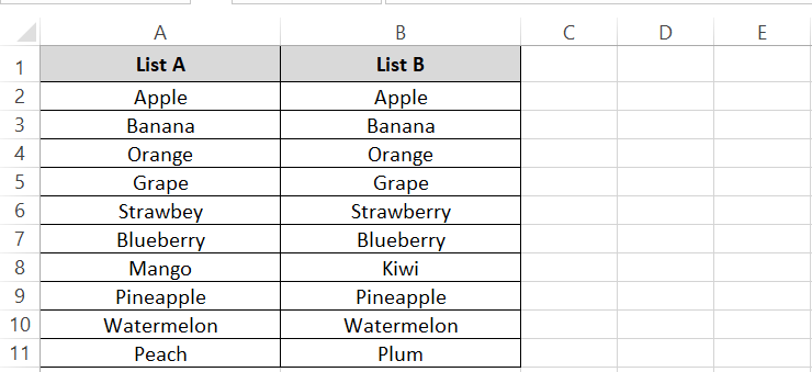
Scanning these lists broadly, looks like both are a clone of each other. To cross-reference them both to see if they are, the simplest method is asking Excel if List A is equal to List B 📃
Agreed? Then let’s do it.
Step 1) Activate a cell in the column next to the second list.
Step 2) In the first cell of this column, write the following formula:
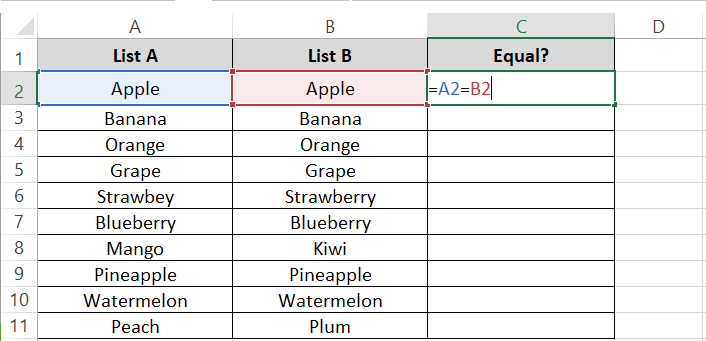
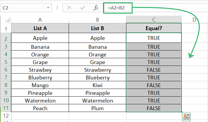
This is a logical formula that checks if A2 is equal to B2 and accordingly returns TRUE (if both the cells are equal) and returns FALSE (if they are not equal).
Step 3) Press Enter.
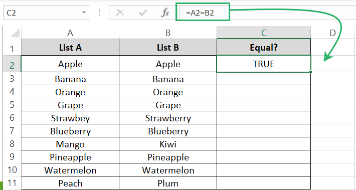
A2 is a perfect match of B2 hence we get TRUE.
Step 4) Drag this formula down until the end of the adjacent column.

Most of the list matches, but certain cells from this list are not the same and we get FALSE for them.
This is how you can quickly compare two lists to find any differences ⌚
Cross Reference two lists in Excel using the IF function
The method to use the IF function to compare two lists is built on the above method of using an equal to the operator (=).
Just wrap the logical condition of A2=B2 into the IF function and define a value_if_true and a value_if_false to get these values returned instead of TRUE / FALSE 🎁
Step 1) Activate a cell in the column next to the second list.
Step 2) In the first cell of this column, write the following formula:
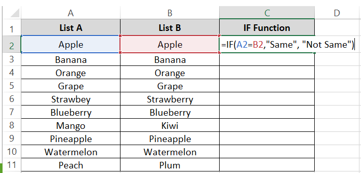
The IF function will check if A2 is equal to B2. If it is, it will return “Same” instead of TRUE. And if both these cells are not equal, it will return “Not Same” instead of FALSE.
Step 3) Press Enter.
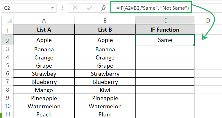
Step 4) Drag this formula down until the end of the adjacent column.
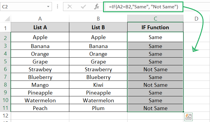
The results are the same as above with the exception that TRUE is replaced by “Same” and FALSE is replaced by “Not Same” 🚀
You can define any other text strings in place of these as you want to be returned.
Cross Reference two lists in Excel using the Row Difference Technique
You can also quickly find how two columns differ by using the Row Difference technique.
Check this out. To cross-reference the two lists in our data to see if they are the same, follow these steps 👇
Step 1) Select both lists.
Step 2) Go to the Home tab > Editing group > Find & Select > Go to Special.
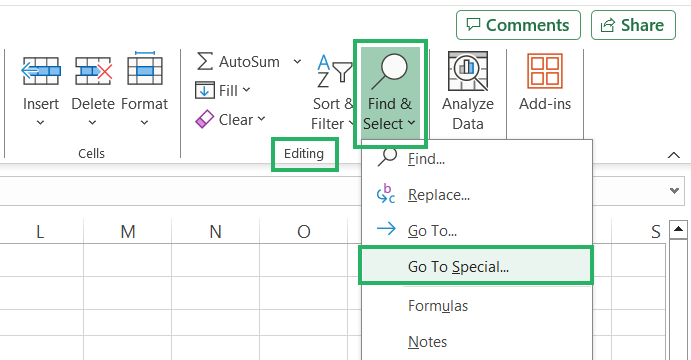
Alternatively, you can press the Ctrl key + G key or just the F5 key to launch the Go to the dialog box and then click on the Special button to launch the Go to Special dialog box.
Step 3) Select the option for Row Differences in the Go to Special dialog box.
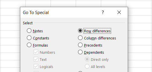
It will select the cells from either of the lists that are different in both columns.
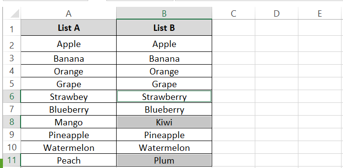
You can then highlight them bold them or format them any way you like to keep track of the differences between both lists.
Cross Reference two lists in Excel using Conditional Formatting
Conditional Formatting is one of my favorite tools from Excel.
You can use it to find differences between two lists in two ways (find the differences or find the similarities) 🤩
Let me show you here.
Step 1) Select both lists.
Step 2) Go to the Home tab > Styles Group > Conditional Formatting > Highlight Cells Rules > Duplicate values.
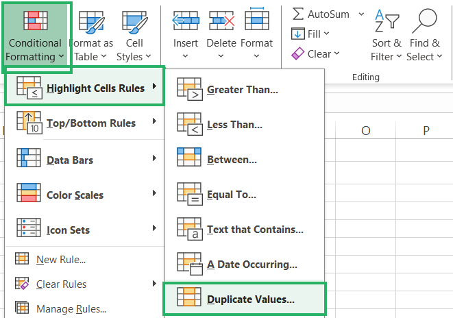
Step 3) From the Duplicate Values dialog box, select Duplicate if you want Excel to highlight the duplicate values from the elected dataset (same values).
Step 4) Set up the font style with which you want these values formatted.
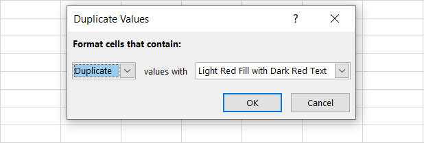
Step 5) Click okay to have these values highlighted from the dataset.

Alternatively, if you want to compare both the lists such that you want to find out the different values from both the lists 📝
Step 1) From the Duplicate Values dialog box, select Unique. Excel will then only highlight the Unique values from the selected dataset (different values).
Step 2) Set up the font style with which you want these values formatted.
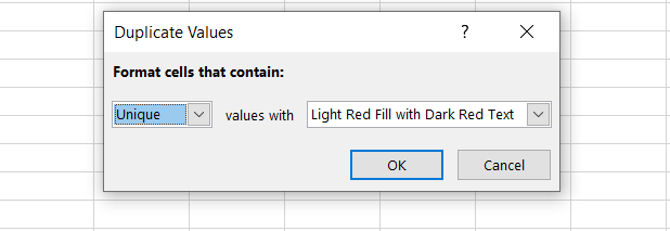
Step 3) Click okay to have the different or unique values highlighted from the dataset.
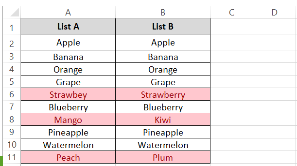
This method allows two-way cross-referencing of data quickly.
Cross Reference two lists in Excel using VLOOKUP
Lastly, all the methods we have seen until now work in the sense that the lists are perfectly synchronized and then the lists are to be compared 📊
Like here, the same names are expected to be written side by side for the equal operator to cross-reference them.
But if a list is ordered such that both the lists are the same but in a jumbled order.
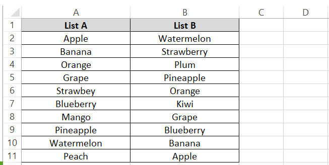
None of the above methods will work to accurately cross-reference such lists.
For such an instance, the VLOOKUP function can help you cross-reference two lists.
Here’s how.
Step 1) Activate a cell in the column next to the second list.
Step 2) In the first cell of this column, write the following formula:
The VLOOKUP function will see if the value in cell B2 appears in the cell range A2:A11. If it does, the same value from the range A2:A11 will be returned, and if it doesn’t, the #N/A! error will be returned 🎯
Since we will drag this formula down to check for all cells of List B, hence we will keep the cell reference for B2 a relative one. But as the range A2:A11 (List A) has to remain constant as we drag the formula down, this will be an absolute reference.
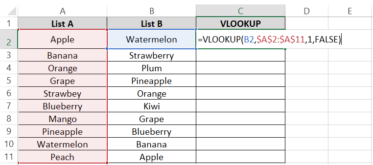
Step 3) Press Enter.
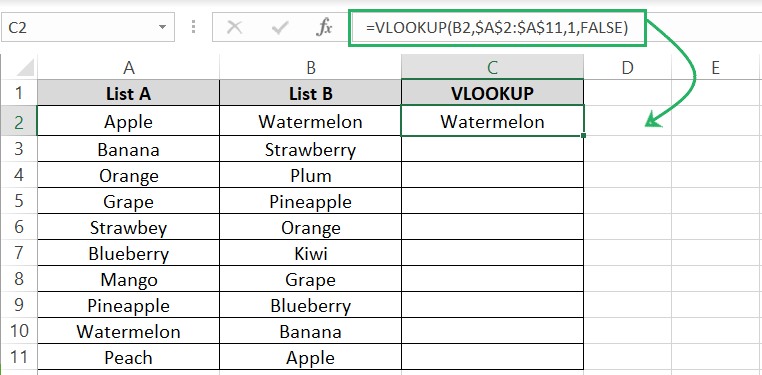
Step 4) Drag this formula down for the whole list.
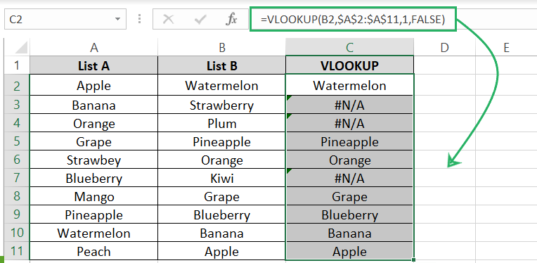
There you go, even though the lists were jumbled, VLOOKUP finds out those items from List B that are different from List A.
If you do not list the #N/A! error on your sheet you can nest the VLOOKUP function in the IFERROR function as below to have any other value returned in its place 🚴♀️
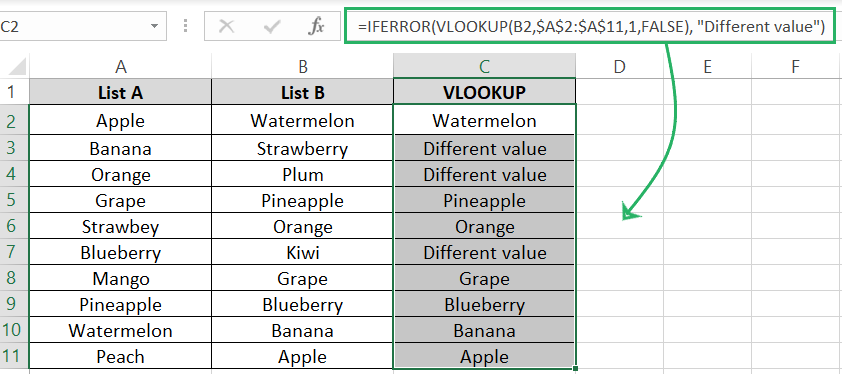
Now for all the items of List B that are inconsistent with List A, we get the result “Different value” instead of the #N/A! error.
Conclusion
In this guide, we have discussed various ways how you can cross-reference two lists in Microsoft Excel. From a simple equal to operator to functions like VLOOKUP, the above guide is a pack of information.
To learn similar other methods to perform comparisons in Excel, check out the following Excel tutorials by Spreadsheeto.
