Excel Date Formula Explained (Change Date Format)
Using dates in Excel can get frustrating sometimes if you do not understand the science that runs behind a date stored in Excel.
There are just so many ways how a date can be presented in Excel. From a short date format to a long date format, to dd:mm:yyyy or mm:dd:yyyy and so many more 📝
However, behind all these dates – Excel has only stored a serial number that starts from 01 January 1900 and keeps counting up until eternity. Learning Excel date formats and their backend settings can ease your Excel jobs involving dates by many folds.
Teaching you about the date format in Microsoft Excel is the core purpose of this guide. It is suggested that you grab your free practice workbook for this tutorial here and continue reading till the end.
Dates in Excel
Look at this date in Excel
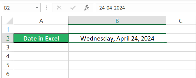
Despite how fulfilling it looks, let me tell you this is just the serial number 45036 in Excel that will show up if I change the format of this cell to General.
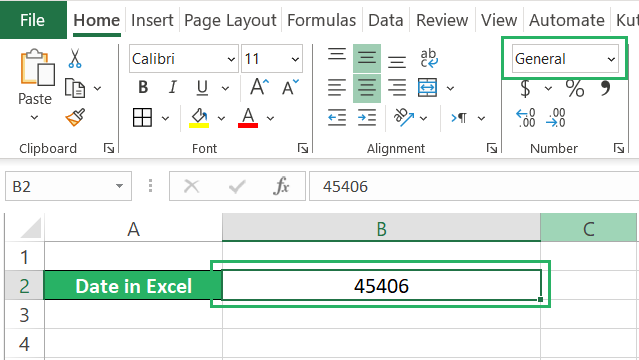
So is the case with all the dates in Excel.
Excel stores all dates as sequential numbers where 1 is equal to 01 January 1900, 2 is equal to 02 January 1900, and so on 📆
20 April 2023 is equal to the serial number 45036 because it is 45036 after 01 January 1900. Hope this explains how the date system of Excel works.
Since Excel knows the first day of the year 1900 as 1 and there’s no concept of negative dates really, Excel doesn’t recognize dates before 01 January 1900.
Choose between a short/long date format
The easiest and quickest way to format a date in Excel is to apply the short date format (if you only want the date) or the long date format (if you want the date + day of the week) to it.
I have some serial numbers here that are basically dates 🏸
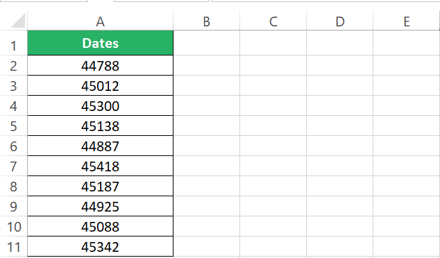
To convert them to dates:
Step 1) Select the cells containing these numbers.
Step 2) Go to the Home tab > Numbers Group > Number formats.

From the number formats drop-down menu, select the short or long date format (based on the date preview that you can see next to it).
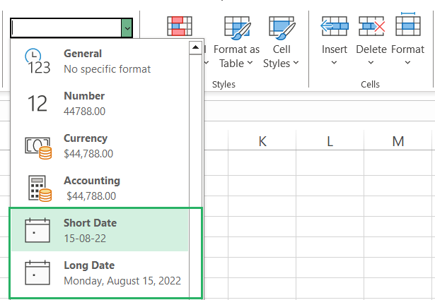
And Tada! Serial numbers will be changed into dates.
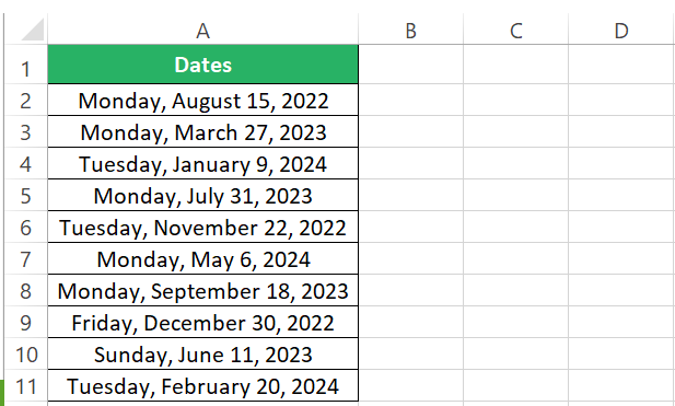
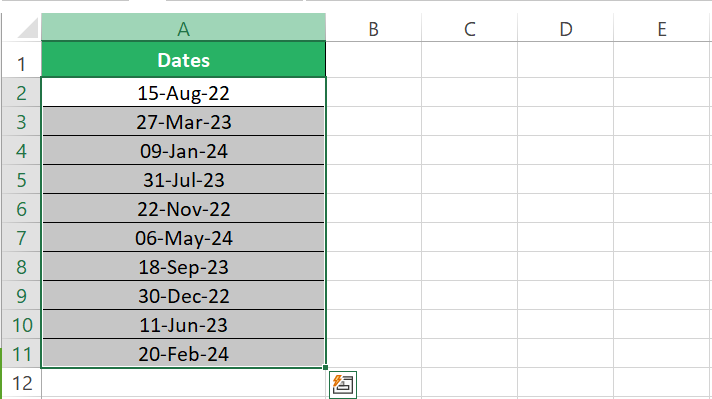
Guess we all converge on the fact that the easiest-to-decode date format is dd:mmm:yy. Excel acknowledges the same and offers the keyboard shortcut [Control key + Shift key + #] to apply this particular date format to any date in Excel ⌨

It doesn’t matter what the date format was applied previously and what your Window settings are, clicking on a cell and pressing Control + Shift + # will convert the date in that cell to dd:mmm:yy format like 15-Aug-22.
Changing the default date format for Excel
To set a different default date format for Excel, you’d need to set it up for your Windows by following the steps below 👇
Step 1) Search for the Control Panel on your PC and launch it.
Step 2) Go to Region.

Step 3) From the Regional settings dialog box, select the Format tab.
Step 4) Set up the date and time format as desired.
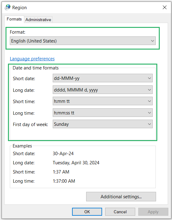
You may also toggle around by clicking on the Additional Settings button to write a custom short and long date format for your Windows.
Choose from In-built date formats of Excel
Excel offers a variety of date formats that you can quickly choose from for the dates populated in your Excel sheet 🧐
Step 1) Select the cells containing dates that you want formatted.
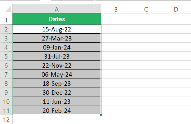
Step 2) Go to the Home tab > Numbers Group > Number formats > More Number formats.
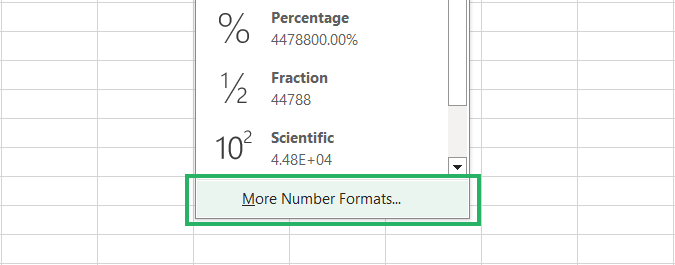
Or just press the Control key + 1 to launch the Format Cells dialog box.
Step 3) From the Format cells dialog box, go to the Number tab and select Date from the Category list on the left.
Step 4) Choose the date format you want applied.
As you select any date format, Excel will show you a preview of how the date looks under that format 🧐
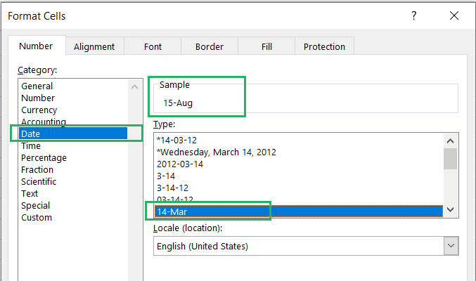
Step 5) Select the date format that fits you the best and press okay.
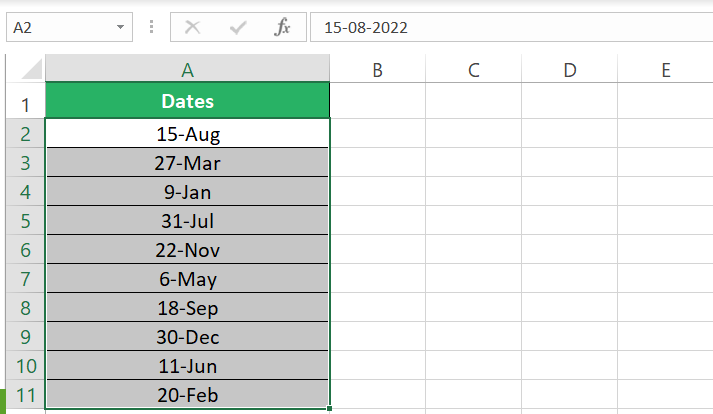
The chosen date format will be applied to the selected cells.
Create a custom date format
Having a wide range of formats at your disposal is great but this must not restrict you. If you don’t feel like settling for the predefined date formats of Excel, you can define the one you like.
Step 1) Select the cells that you want formatted.
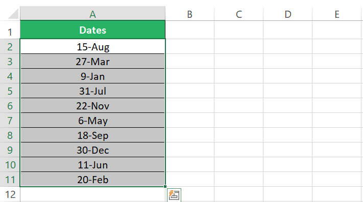
Step 2) Press Ctrl + 1 to launch the Format Cells dialog box.
Step 3) From the Format cells dialog box, go to the Number tab and select Custom from the Category list on the left.
Step 4) In the Type box, type in the date format you want.
As you write up a date format, Excel will show you a preview of how the date looks under that format 🙈
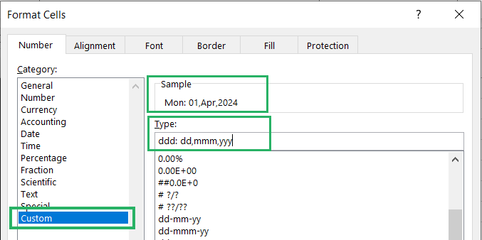
Step 5) Once you have written up the custom date format, press okay.
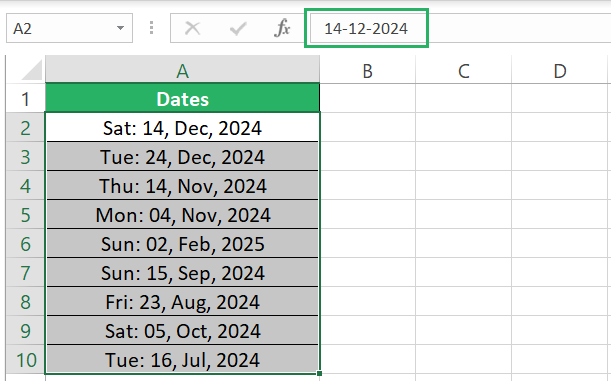
And you’d see that date format applied to all the selected cells.
Dates format with different locales
It is often the case that you want dates displayed in another language or country’s format (other than English) 🏳
Can this be achieved in Excel? For sure – the locale code of the data needs to be set up.
Step 1) Select the relevant cells with dates.
Step 2) Press the Control key + 1 to launch the Format Cells dialog box.
Step 3) Go to Custom from the Category list on the left.
Step 4) Write up whatever date format you desire.
Step 5) Just before the date format, include the locale code of the region whose format/language you want to adopt.
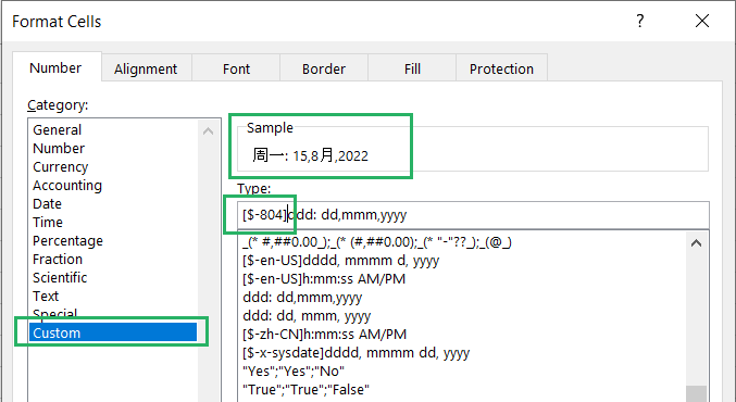
Step 6) Press okay to have the date formatting of that specific locale applied to all the selected cells.
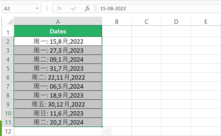
You can find the locale codes for all languages from multiple online sources.
Change the date format using the TEXT function
The TEXT function is meant to take a value from you and return it in the format you specify.
For example, I have some dates listed in Excel 📚
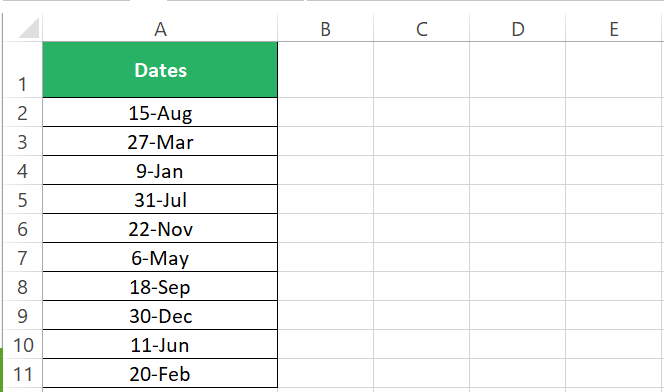
I want these to be formatted as dd-mmmm-yy (in other words as 01-January-2024).
One of the ways to do this is to go to Format Cells and then select the desired format to be applied to these cells.
Another way to achieve these results is using the TEXT function. Check this out.
Step 1) Write the TEXT function as follows:
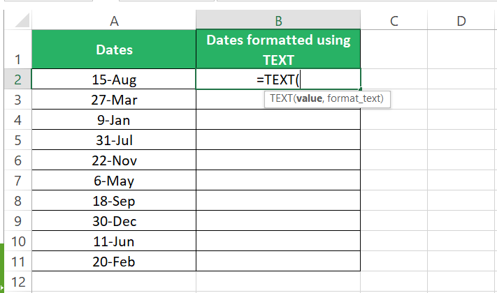
Step 2) As the first argument, write the cell that contains the dates to be formatted.
Step 3) For the second argument, specify the format in which you want the date formatted within double quotation marks.
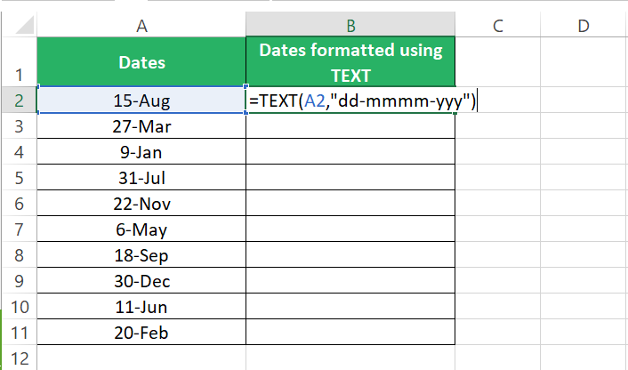
Step 4) Press Enter
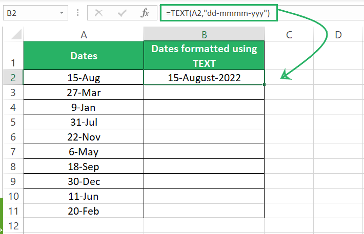
Step 5) Drag the same formula down the whole list.
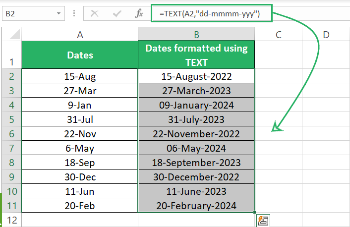
The whole list of dates adapts to the dd-mmmm-yyy format.
Create dates using the DATE function
Formatting dates as dates in Excel is a task – I must say. You might make a small mistake in writing up the date, and Excel will fail to recognize it as a date.
This is particularly important if you are writing date within a formula or if you need to refer to it within other formulas 🎯
Luckily, you can write up any date (in a format recognized by Excel) by supplying the year, month, and date number to a function that we call the DATE function.
It is simple and foolproof.
Step 1) Write up the DATE function as below.
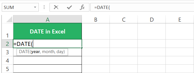
Step 2) Supply the year, month, and date numbers. For example, to write up the date 12-Apr-2024, I’d write the DATE function as:
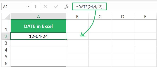
Excel writes up it as a date.
Normally, if you write up the date 24-04-12 in a cell in Excel, you might mean 20-April-2024, and Excel may take it as 04 December 2024 or 24 April 2012 (you never know). Depends on the default date format of Excel.
This might have a take on the accuracy of your data 🏍
Convert dates formatted as text using the DATEVALUE function
Just like the name says, the DATEVALUE function returns the numeric value for a date (as Excel knows it).
You’d need this function particularly when you import data from External sources (like from the web or any .csv file). Dates within the imported date are often taken by Excel as text values.
Like here 💡
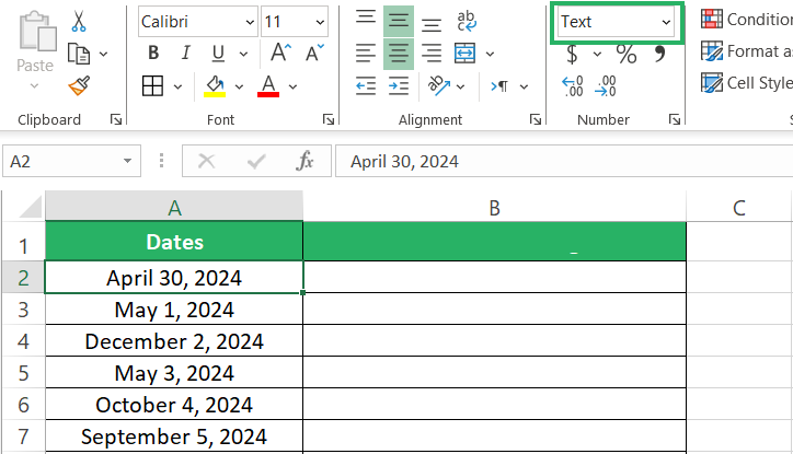
The problem with this format of dates is that you cannot use them in your formulas as dates (adding or subtracting dates from them). You can also not format them to different date formats as Excel doesn’t recognize this date as a serial number but as a text string.
To fix this problem:
Step 1) Write the DATEVALUE function as below.
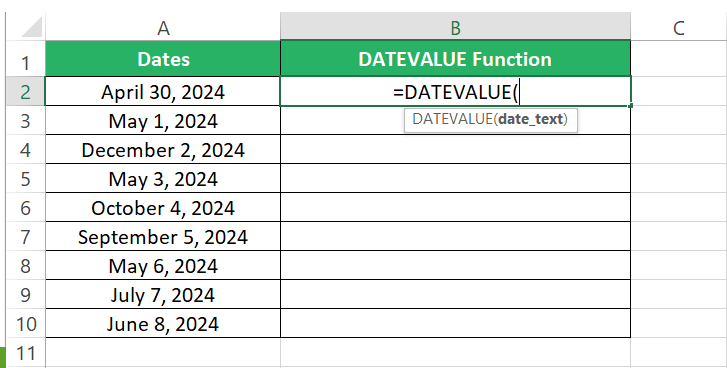
Step 2) Supply the cell reference that contains the dates formatted as text to it and hit enter.
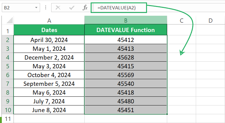
Excel will convert the given text formatted date to the numeric value equivalent to it.
Step 3) You can then apply whatever date formatting you want to these numbers.
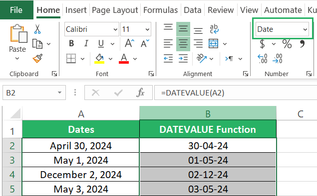
In some cases, this workaround might not help you fix dates as the DATEVALUE function returns the #VALUE! Error. For such a situation, it is suggested that you remove all the formatting from these dates by applying the general formatting 👀
And then try applying the desired date format to it.
Conclusion
The article above is a complete package of all the top methods that you can use to change date formats in Excel. From using in-built date formats offered by Excel to customizing your date format. You can do so by using the Format Cells option or by using Excel’s versatile functions.
All in all, there’s so much about working around with dates in Excel that we are yet to explore. Make sure to check out my following Excel tutorials that cover these areas.
