How to do RANK IF in Excel to Rank With Condition
Ranking values in Excel is something very common. And with the RANK function, that’s not even a problem.
However, if you want to perform a conditional (or criteria-based) ranking in Excel, this might be a little problem at first 😣
That’s because Excel doesn’t offer an in-built RANKIF function. But this won’t stop us!
The RANKIF function can be substituted by a tweaked version of the COUNTIFS function. Let me take you through the guide below that will teach you how to do this.
So continue reading and download our free sample workbook here as you slide down 👇
Table of Contents
Use RANK IF to rank with criteria
Here we have a dataset that lists the sales from different months.
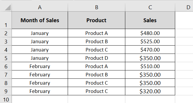
Can we quickly rank these sales? The Excel RANK function will do that in a blink 😎
= RANK (C2:C9)
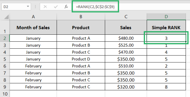
That was fast! But now what if I want to rank the sales for each month? The highest to lowest sales for January and February, both.
Now that’s what we call conditional ranking. It becomes conditional as we want the rank of the sales but only within a specific month 💪
For conditional ranking, we need the RANKIFS function. And as Excel has no such function, here’s a workaround for it.
- Write the COUNTIFS function as follows:
= COUNTIFS (
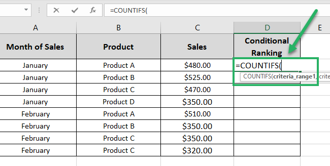
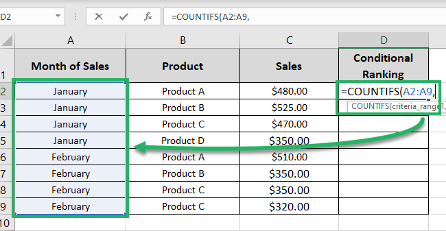
- As the first criteria range, define the range for the first criteria.
Our first criterion is the month of Sales, so we are referring to the column of months 📅
= COUNTIFS (A2:A9
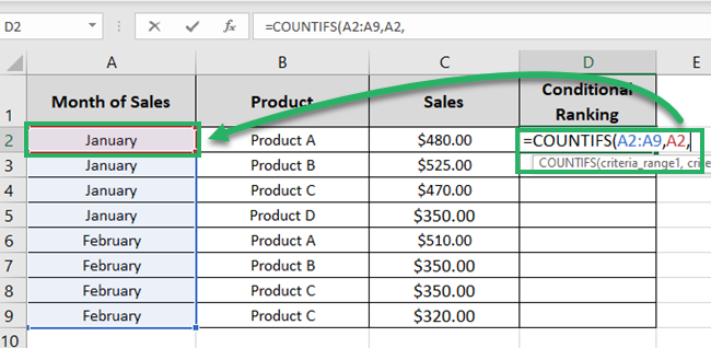
- As the first criterion, refer to the month whose sales we want to be ranked.
As we need the sales for each month, so we will refer to the respective cell containing the month as the criteria.
= COUNTIFS (A2:A9, A2
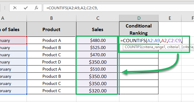
- As the second criteria range, define the range where the second criterion is to be checked.
Our second criterion will help us rank the sales from highest to smallest so we are referring to the column that contains sales 📝
= COUNTIFS (A2:A9, A2, C2:C9
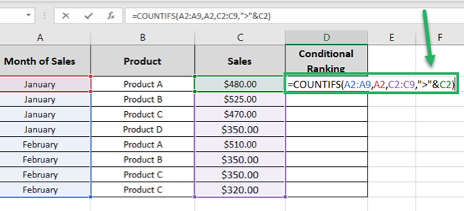
- Define the second criterion. The second criterion will simply be “greater than the corresponding sales”.
= COUNTIFS (A2:A9, A2, C2:C9, “>”&C2)
Pro Tip!
Note that we have used the greater than operator (>) enclosed in double quotation marks as “>”.
That’s how you specify conditions for COUNTIFS using operators. To use operators with a cell reference, we must use an ampersand (&) in between. So with a cell reference (say C2), the criteria above become:
The operator enclosed in double quotation marks + an Ampersand + the cell reference
“>”&C2
- Close the parenthesis for the COUNTIFS function.
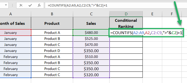
- Write +1 after the function as shown here.
= COUNTIFS (A2:A9, A2, C2:C9, “>”&C2) + 1
Pro Tip!
Why did we write +1 at the end ❓
The simple COUNTIFS will count the number of sales that pertain to the corresponding month and that are greater than the corresponding sales.
But we don’t want the count of such sales, we want the rank of sales. For that, we add +1 to the above formula. The rank of each sale for a month will be “The count of sales of the month that are higher than that sale + 1”.
- Hit Enter!
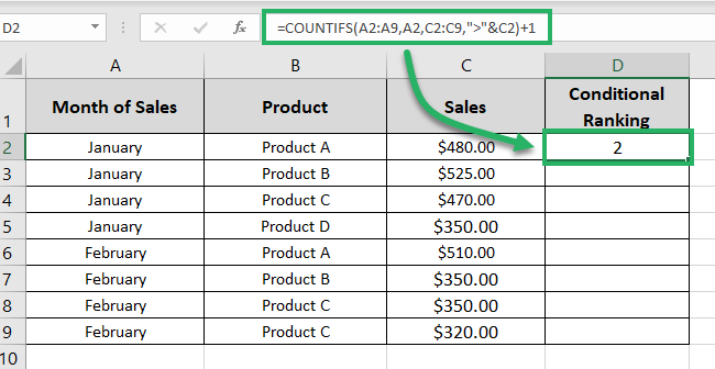
The sale of $480 ranks at position 2. This means it is the second-highest sale from January 🔎
- Go to the formula bar.
- Take your cursor to each range reference (A2:A9 and C2:C9) and press the F4 key to turn them into absolute references.
= COUNTIFS ($A$2:$A$9, A2, $C$2:$C$9, “>”&C2) + 1
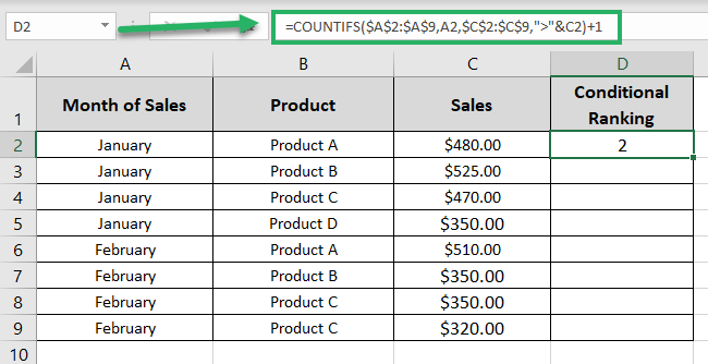
This is because Excel will update the cell references as we drag and drop them down across the next cells. We want the cell reference for the first criteria (month) and the second criteria (sales higher than the current sale) to update. But the range must remain constant 💡
- Drag and drop the results to the whole list of sales.
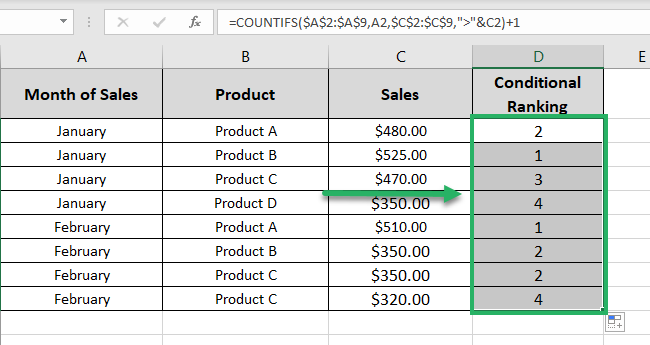
With this, we have all the sales (for each month) ranked. Want to double-check these results for accuracy? Let me sort the ranks in ascending order here.
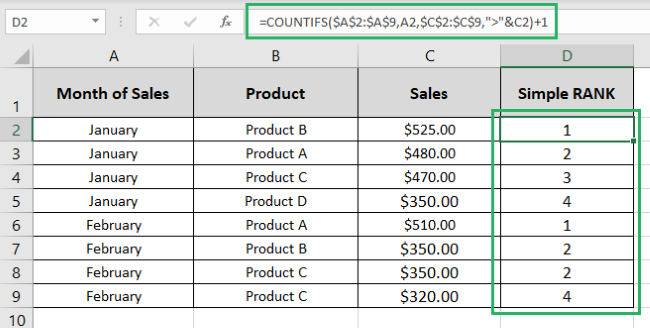
Woah! That makes perfect sense. The numbers and the ranks align 🧐
But what’s that? For February, there’s no 3rd rank but two times the 2nd rank – and then the 4th rank straight?
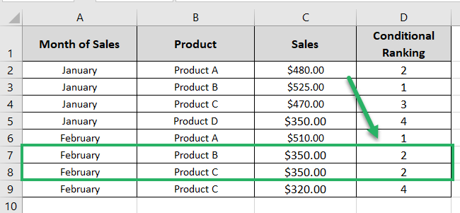
That’s because in February we have two sales for the same amount of $350. So Excel ranked them both at the 2nd Position. And the amount next higher to $350 (i.e. $380) is ranked as 4th and not 3rd 🚩
This is the same as the general behavior of the RANK function.
Use RANK IF to rank with criteria in reverse order
In the example above, we’ve seen how you can use the COUNTIFS function to perform conditional ranking (in descending order i.e. highest to lowest).
But what if we want to perform conditional ranking in reverse order? In other words, in ascending order (lowest to highest). That’s equally easy to be done 🪁
Check it out here. Same previous example – however, this time we want to rank the sales for each month in reverse order.
We want the lowest sales for January ranked at 1st position. The sales higher to it on the 2nd and so on.
Let’s do that here:
- Write the COUNTIFS function as follows:
= COUNTIFS (
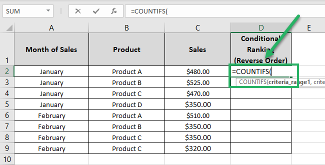
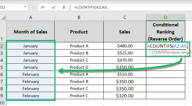
- Define the range for the first criterion.
Our first criterion is still the month of Sales so, we are referring to the column that contains the month names.
= COUNTIFS (A2:A9
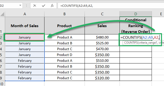
- Define the first criterion.
We need the reverse ranking for sales for each month, so our first criterion will be the corresponding month for that sale.
= COUNTIFS (A2:A9, A2
- Next, define the range where the second criterion is to be checked.
Our second criterion will rank sales so referring to the column that contains sales 💰
= COUNTIFS (A2:A9, A2, C2:C9
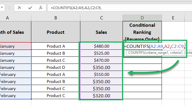
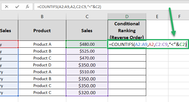
- Define the second criterion. This time, the second criterion will be “Lesser than the corresponding sales“.
= COUNTIFS (A2:A9, A2, C2:C9, “<”&C2)
Pro Tip!
This step makes the difference. To perform ranking in a simple order, we wrote the criteria using the greater than operator (>) 🚴♂️
To perform the ranking in reverse order, we will write the criteria using the lesser than operator (<). This is how the criteria will look like:
“<”&C2
Nothing but the operator is changed from (greater than) > to (lesser than) <.
- Close the parenthesis for the COUNTIFS function.
- Write +1 after the function as usual.
= COUNTIFS (A2:A9, A2, C2:C9, “<”&C2) + 1
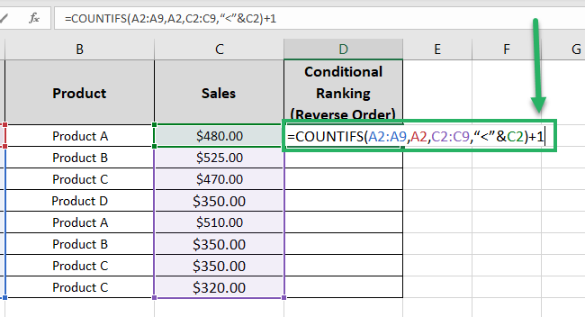
- And you’re all good to go – Hit Enter 🎯
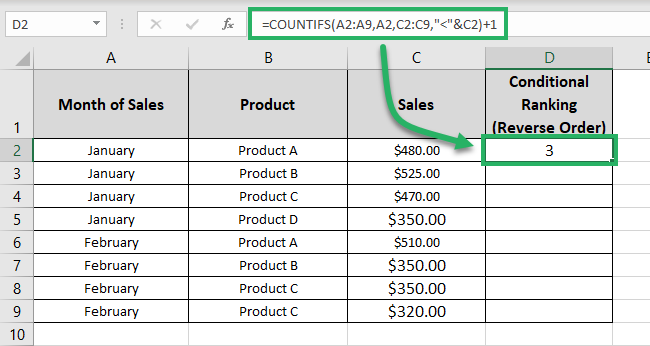
This time the first sale of January i.e. $480 ranks at the 3rd position. This means it is the third lowest sale from January.
- Turn the range references in the above formula into absolute references (like below):
To do this, go to each cell reference in the formula bar and press the F4 key.
= COUNTIFS ($A$2:$A$9, A2, $C$2:$C$9, “<”&C2) + 1
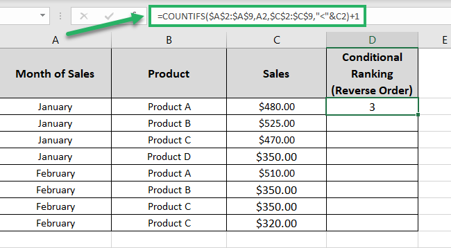
- Drag and drop the results to the whole list of sales.
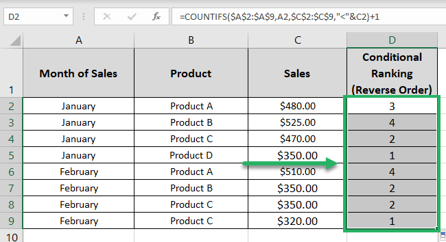
Note that this time the sales are ranked in a reverse (ascending order). The lowest sale is ranked at 1st position, and so on 🥇
That’s it – Now what?
Woah! Though Excel doesn’t offer an in-built RANKIF function, you can still perform conditional ranking in Excel using the COUNTIFS function. Isn’t that great?
The guide above teaches us how we can use COUNTIFS to rank values in Excel based on a criterion. And also how to rank them in reverse order with the same criteria 😍
This tells about the versatility of this spreadsheet program. Even if it misses out on any function, you can still make it work by tweaking other functions.
Interestingly, Excel has a wide variety of functions that can be used to achieve different results. To start, I suggest you go with the SUMIF, IF, and VLOOKUP functions.
How to learn them? Click here and register for my 30-minute free email course now to get your hands on them (and much more).
Other resources
You’ll be great at using the COUNTIFS function to perform conditional ranking if you know how to use the basic RANK function in Excel.
And once you have mastered the basic and the conditional RANK functions in Excel, learn more about the possible problems the IF function might pose.
