Number Formatting in Excel: Step-by-Step Tutorial
We all know how to apply the basic numeric and text formats to cells in Excel.
But do you know how you can add a desired number of decimals, scientific notations, currency symbols, and similar formats in Excel with only a click?
No? This article is for you. It delves into the details of number formatting in Excel. 🤩
Keep reading till the end, and download our free sample workbook here before you scroll down.
Table of Contents
What are number formats?
Type something into a cell. What is its format?
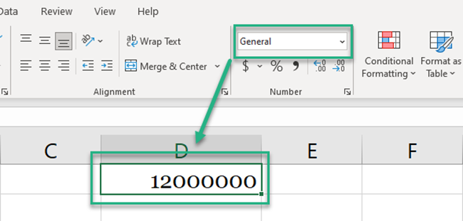
By default, all cells of Excel will have the General format applied.
However, type in a big number that exceeds the size of the cell, and Excel would give you back something like 1.2E+12.
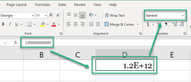
What is this? A scientific notation. Under General format, Excel replaces a number too big to fit the cell with its scientific notation.
To turn it into a number, change the format to ‘Numbers’ and adjust the cell size.
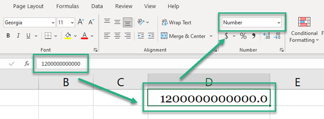
Check the formula bar to note how the number remains the same under both formats i.e. 1200000000000.
What changes is only the visual representation of the said number in Excel (decimal places added).
That is how formats work in Excel.
And you can change the format of a number with a mere click. Excel offers many number formats with useful variations to them.
Thousands separator
In the image below we have different numbers.
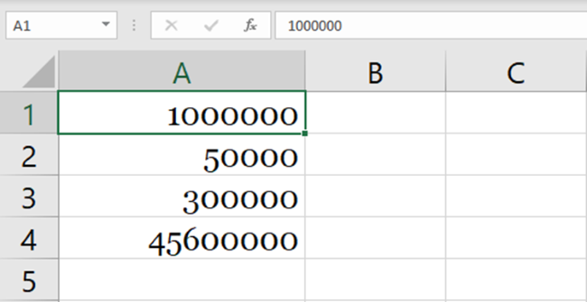
By now, it only seems like a number that is hard to read. Maybe that’s because it doesn’t yet have 1000s separators (any commas) to it.
- Select the cell.
- Go to Home > Number

- From the menu, go to More Number Formats
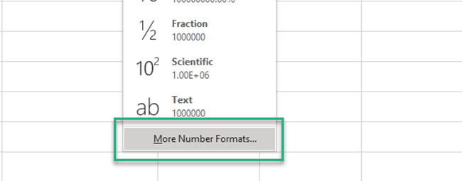
This launches the Format Cells dialog box.
You may use the keyboard shortcut (Control Key + 1) to launch the Format Cells dialog box.
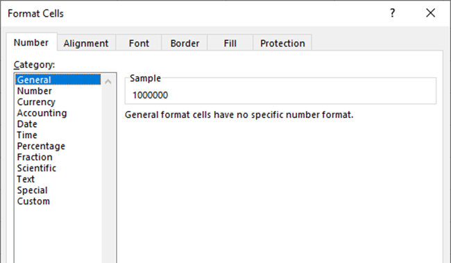
- Go to Number Format.
- Check the ‘Use 1000 Separator’ box.

- Here are the results.

A shortcut to add the 1000s separator: Go to Home > Number > click on the comma symbol

However, this changes the number format to the Accounting format.
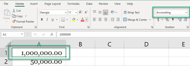
Controlling decimals
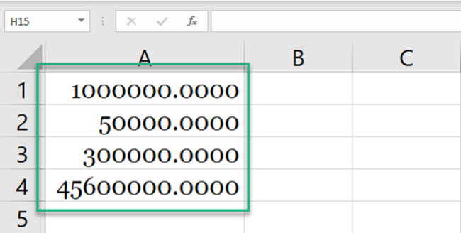
In the same example, as above, there are two decimals to the number.
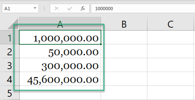
But you want four decimal places to this number. How can this be done?
- Select the cell.
- Go to Home > Number > More Number Formats

- From the Format Cells dialog box, go to Number Format.
- Adjust the decimal places to four.
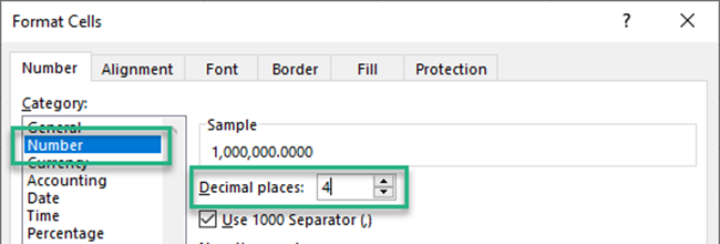
- Here are the results.
A shortcut to adjust decimal places. Go to Home > Number > Add decimals button

With every click, Excel adds another decimal position to the number.
The button with a right-headed arrow reduces a decimal position.
The button with a left-headed arrow adds a decimal position.
Show as percentage
Here is a decimal number that we want to be converted into a percentage.
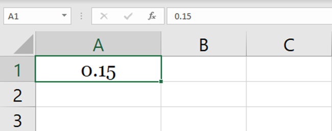
To do this:
- Select the cell.
- Go to Home > Number > More Number Formats

- From the Format Cells dialog box, go to Number Format.
- Click on Percentage.
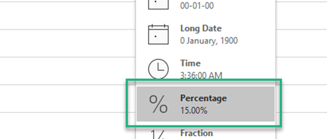
- Adjust the decimal places as desired.
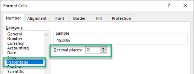
- Here are the results.

A shortcut to convert a number into a percentage. Go to Home > Number > Click the % symbol

Number formatting presets
Excel offers a wide variety of number formatting presets. (You must’ve had a slight idea of that by now.)
These range from currency to accounting to dates and whatnot.
Let’s look into each of these formats below.
General number format preset
The general number format of Excel is the default format of any value in Excel.
All values in all cells of Excel will have the general number format by default.
- To apply the general format to any cell in Excel, select that cell.
- Press the Control key + 1 to launch the Format cells dialog box. That’s a handy shortcut 😊.
- Choose the ‘General number’ format.
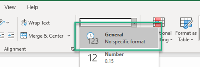
- Values formatted as general numbers are displayed just the way they are.
Pro Tip!
Under the General number format, if the cell is not wide enough to contain a number, Excel would:
- Round a number with decimals to lesser decimal places; or
- Use scientific notation to express the number; or
- If the cell is too small to fit in the scientific notation for the number even, display a series of hashes only.
Number format preset
The Excel number format is used for simple numeric values
To apply the number format to any cell:
- Select the cell.
- Go to Home > Numbers > Drop Down Menu and click on Number Format.
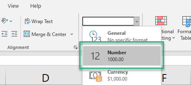
The number format allows users three further variations to the final value:
- The decimal places. You can adjust decimal places to any desired number.

- The 1000 Separator. Check the box if you need 1000s separators to the value.
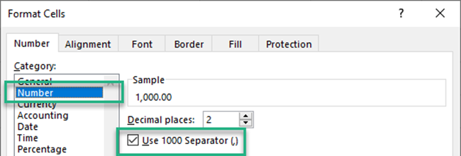
- The format of negative numbers. This could be in two colors (black or red) and enclosed within brackets or with a minus sign.
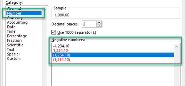
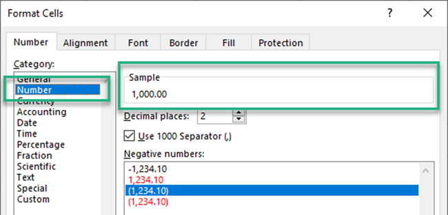
The Sample box gives a preview of what the final value may look like.
Must Note:
Under the Numbers format, if you type a number in a cell that is too big to fit in the cell, Excel might return a series of hashes only.
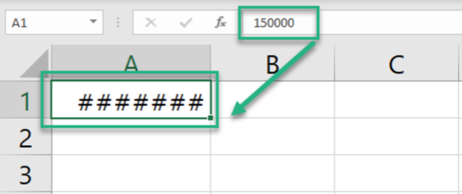
In such a case, one must know that the problem simply lies within the size of the cell. (that is too small to fit in the cell value).
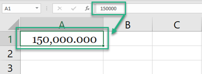
To work this out, increase the width of the column until it is wide enough to fit in the cell value.
Currency format preset
The Currency format is used to denote currencies.
To format a number as currency:
- Go to Home > Numbers > Drop Down Menu > Click on Currency.
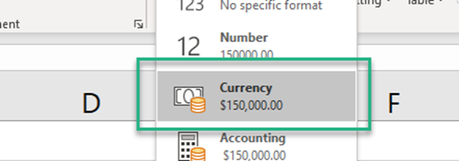
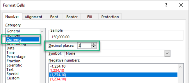
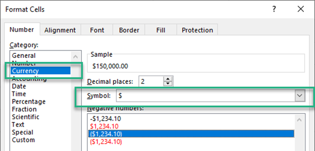
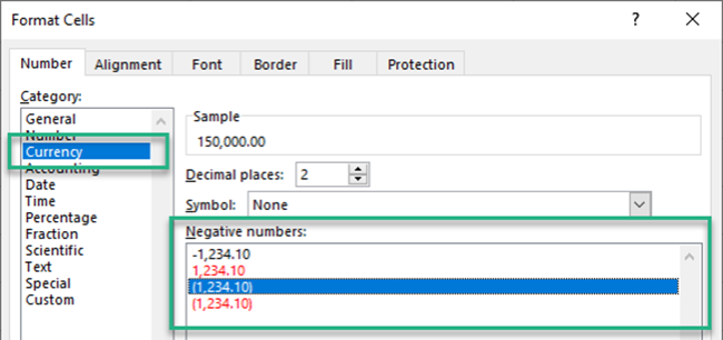
It allows you to adjust three options to your desire:
- The decimal places.
- The currency symbol.
- The format of negative numbers. This could be in two colors (black or red) and enclosed within brackets or with a minus sign.
Here is what a currency formatted number looks like.

Date format presets
There are two date formats offered by Excel – short date and long date.

To format a number as a date, go to Format Cells and choose the date format you’d want to be applied.
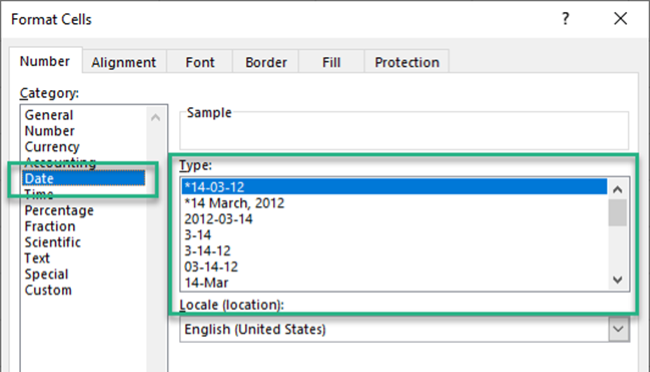
Excel offers a wide variety of formats for dates and days.
Here is how the date format works.
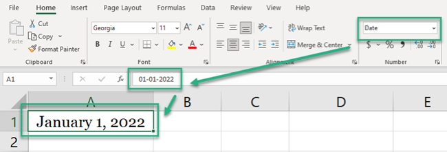
Pro Tip!
Type any number into Excel and apply the date formatting to it. Excel turns it into a date.
This is because Excel recognizes each date as a number. Where 1 is equal to 01 Jan 1900, 2 is equal to 02 Jan 1900, and so on.
Accounting format preset
Next is the accounting format preset.
This format is relevant when you’re working with financial data. For example, while preparing financial statements, forecasts, or similar reports.
To apply accounting format to a number:
- Go to Home > Numbers > Drop Down Menu > Click on Accounting Format.

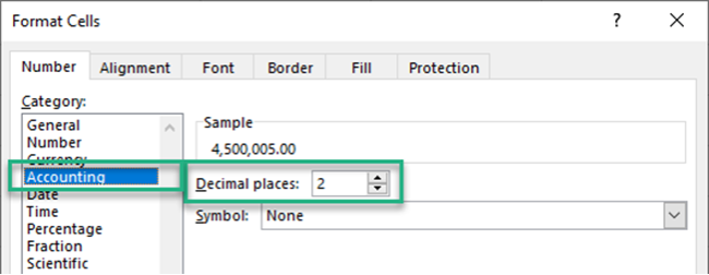
It allows you to adjust two features to your desire:
- The decimal places.
- The currency symbol.
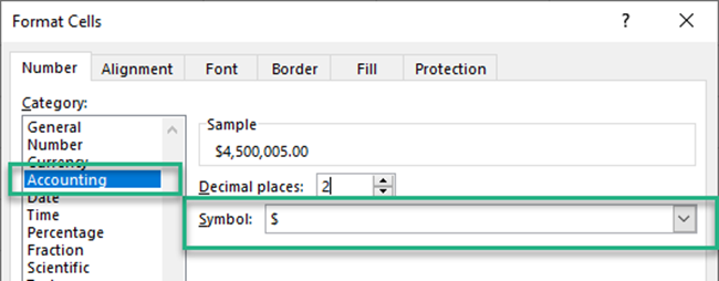
Here is what an accounting formatted number looks like.
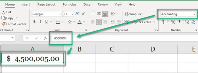
Under the accounting format, 1000s separators and currency symbols are added by default. And negative numbers are enclosed in parenthesis i.e. $ (1925.60) etc.
Time format preset
Excel also offers a wide variety of ways how you may represent times in Excel.
To apply the time format, go to Format Cells and choose the time format you’d want to apply.

You can format it to be displayed as HH:MM:SS or any other way you like.
Here is how the time format looks in action.
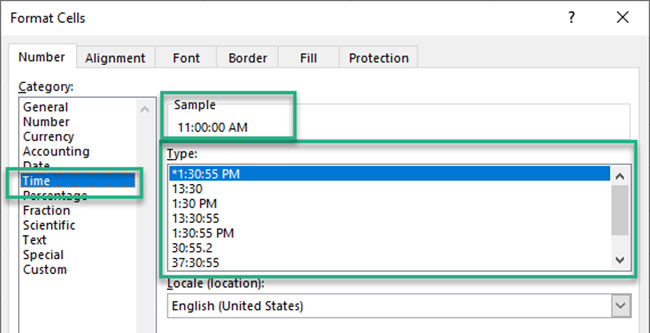
Formatting shortcuts
There are plenty of shortcuts on how you may quickly format cell values in Excel.
You can format numbers by using these keyboard shortcuts. Simply select the cell (or cells) where you want the formatting applied and use the shortcuts below.
- Control Key + Shift Key + ~ : Applies the General format
- Control Key + Shift Key + ! : Applies the Number format
- Control Key + Shift Key + $ : Applies the Currency format
- Control Key + Shift Key + % : Applies the Percentage format
- Control Key + Shift Key + ^ : Applies the Scientific notation format
- Control Key + Shift Key + # : Applies the Date format
- Control Key + Shift Key + @ : Applies the Time format
All of these are shortcut keys and only apply the default formats (like the default two decimal places or HH:MM:SS AM/PM format etc.)
Custom formatting
Tired already? However, the number formats list has yet not come to an end.
The last and the most important number format of Excel is the Custom Format.
Under this format, you can customize a number format as needed.
- Go to Home > Numbers > Drop Down Menu > More Number Formats.
- Click on Custom Format.
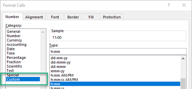
- Under the custom formatting, you see different formats.
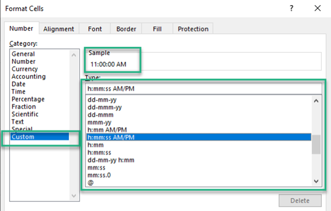
- To create a custom number format, choose the format that closely matches what you are looking for.
- Customize it as needed (keep an eye on the sample to see if you’ve reached your desired format).
- And save your custom number format.
That’s it – Now what?
Like all the amazing tools offered by Microsoft Excel, number formats are a whole toolkit in itself.
There’s so much to explore, and this article only gives you an idea of how you can come up with different visual representations of the same value.
Not only that, but if you fail to find the format you’re looking for – you can customize one for yourself. That’s where the possibilities become limitless.
Want to learn further? Learn the core functions of Excel including the VLOOKUP, SUMIF, and IF functions.
You need not go any further to master these functions. Click here to sign up for my free 30-minute email course that will take you through these and many more functions in no time.
Other resources
This article only sets the foundation for number formatting in Excel. If you liked reading this article, we bet you’d love to know more.
Learn how to Use Superscripts and Subscripts in Excel and How to Clear Excel Formatting.
