Freeze Panes in Excel: How to Freeze Rows and Columns
Freezing here means locking particular rows/columns of Excel in place to enhance the readability of a worksheet.
By freezing panes rows/columns in Excel, you can still view them when you scroll to other parts of the worksheet 🧐
The guide below will help you learn how to freeze (and unfreeze) rows and columns in Excel. So stay tuned, and do not forget to download our sample workbook here to practice along with the guide.
Table of Contents
How to freeze a row in Excel (any row)
Coming straight to the topic – so how can you freeze a row in Excel? See here 👇
The image below has a long list of data for many employees of a company.
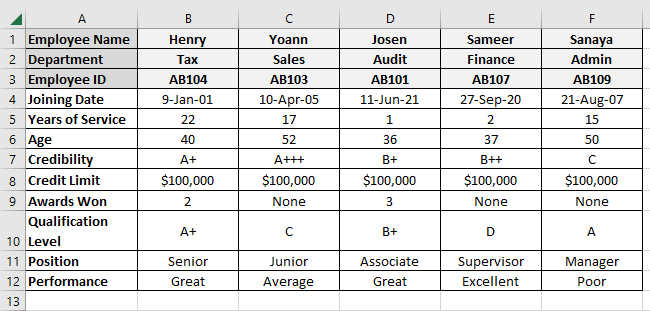
Now as I scroll down the worksheet, I’d miss out on the headers. So I will be able to view the data but, I might not understand it well without the headers.
For example, as I scroll down to Row 6, I can not see the employee’s name, department, and number. So although I can look into the age of each employee, I can’t readily see the name of the employee to which it relates.
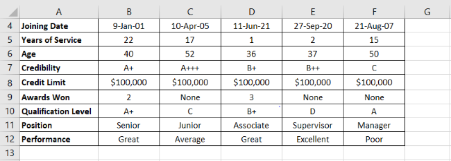
To help this situation, we need to lock the top 3 rows for the name, department, and ID of employees. You can do this by following the steps below:
- Select the row below the last row to be locked (Row 4 in our case). To select it, click on Row Header 4.
We want the first three rows locked. So, the row immediately below the last row (3rd row) that we want to be locked in is Row 4 🔒
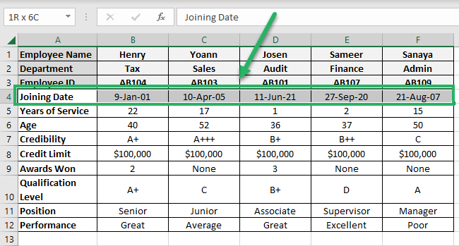
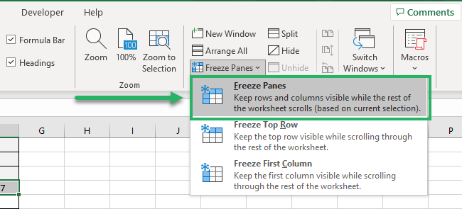
- Go to the View tab > Freezing Panes

This will launch many a menu of options.
- Click the Freeze Panes option.
Pro Tip!
You can also select Row 4 and press the Alt key > W > F > F 👌
Excel freezes the first 3 rows. Scroll down the list to see that the first 3 rows are locked in place.
For example, if we want to scroll down to Row 10, the worksheet will look like the one below.
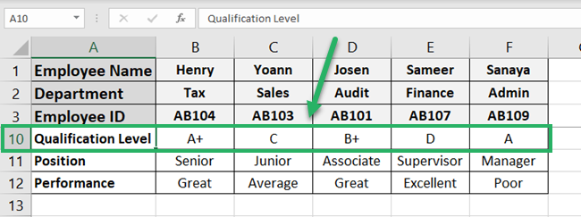
No matter how much you scroll down now, the first 3 rows of your worksheet would not move 🥶
Freeze top row
If you know how to freeze rows in Excel, freezing the top row only is nothing new 🆕
In the same dataset as above, to freeze only the top row (employee names), do as follows:
- Go to the View tab > Freezing Panes

- From the drop-down menu, select the second option to freeze the first row only.
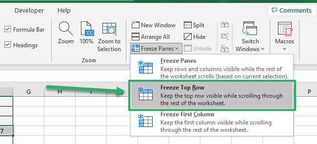
Alternatively, use the keyboard shortcut: Alt key > W > F > R.
Excel freezes the first row only. Scroll down the list to see that the first row is locked in place.
Let’s scroll down to Row 9 to see what the worksheet looks like.

As we scroll down to Row 9, the first row remains visible ✨
How to freeze columns
We have seen how to freeze rows in Excel. And now it’s time we move on to freezing columns.
Hint: It’s just the same as freezing rows 👏
So we are back with our dataset as above. This time let’s freeze the first column (Column A) that contains the description for each detail. To do that.
- Select the column immediately after the column is frozen.
As we want to freeze Column A, we must select Column B.
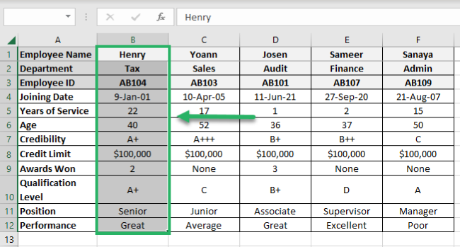
- Go to the View tab > Freeze Panes.
- From the drop-down menu, select the first option Freeze Panes.

As Column A is the first and leftmost column, you can also select the third option “Freeze the First Column”. The results would be the same.
However, if you want to freeze multiple columns, follow the steps above and click on the option to freeze panes 👆
Excel will freeze Column A in its place.
- Scroll to the right to see Column A locked.
For example, we have scrolled up to Column D, and here is what the worksheet looks like.
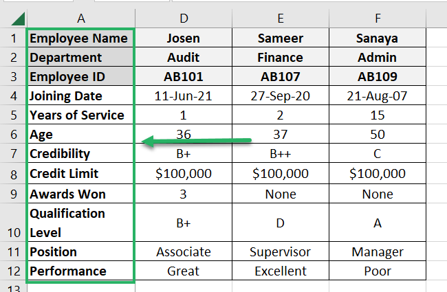
Easy and similar to freezing rows, isn’t it 🚀
Freeze rows and columns at the same time
All good with freezing rows and columns individually. Time for some advancement.
The dataset remains the same. But this time, let’s try to lock multiple rows and columns together.
We will freeze the first two columns (Columns A & B) and the first three rows (Row 1 to 3) together 🧊
Pro Tip!
The entire science for freezing rows and columns together lies within selecting the right cell before we freeze panes.
To freeze rows and columns together, select the cell that falls in the row and the column immediately after the last row and the last column to be frozen.
In our example, the last column that we want to freeze is Column B. The immediately next column to Column B is Column C.
And the last row that we want to freeze is Row 3. The immediately next row to Row 3 is Row 4.
So we will select Cell C4 (which falls at the intersection of Column C and Row 4) 4️⃣
- Select Cell C4.
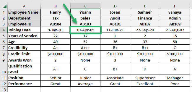
- Go to the View Tab > Freeze Panes.

- From the drop-down menu, click on the Freeze Panes command.
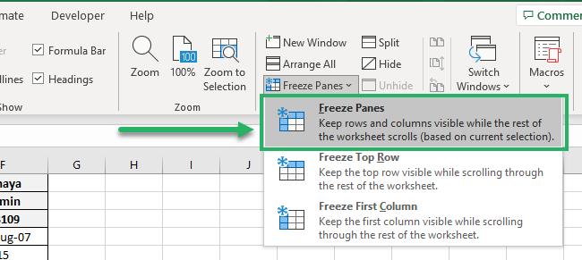
We’re done. Scroll across the sheet, and you’ll notice that Columns A & B and Row 1 to 3 are frozen.
Like the image below, we have scrolled to the right up to Column E. And to the bottom up to Row 9.
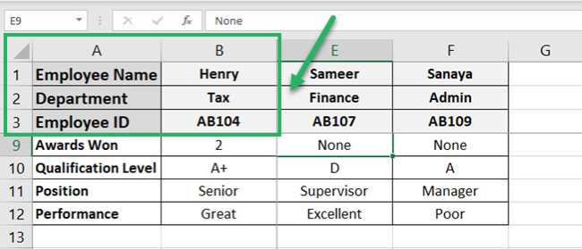
But the frozen rows and columns are still locked and are visible 🔐
Unfreeze panes
Everything that you do in Excel can be undone – no worries.
So if you have your panes (rows or columns) frozen, they are not frozen forever. You can still melt them back 🔥
In the example above, we have the first two columns (Columns A & B) and the first three rows (Row 1 to 3) frozen.
To unfreeze them:
- Click anywhere in your sheet.
- Go to the View Tab > Freeze Panes.

- From the drop-down menu, click on the first option to Unfreeze panes.
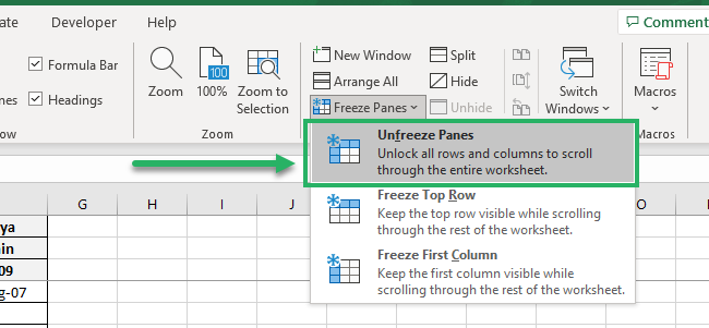
And that’s it. Scroll through your worksheet to see the panes are no more frozen.
You can freely navigate to any part of your sheet 🚴♀️
That’s it – Now what?
Now you know all about freezing rows and columns in Excel. Must have found that easy, didn’t you 💪
Exploring the features of Excel is always fun. And if you are on the journey to explore Excel features, this journey is not coming to an end anytime soon.
Excel has a huge variety of features and functions. Starting from a function as simple as the SUM function to super advanced ones. Mastering Excel functions is the fastest and the only way to become an Excel expert.
Want to start learning already? I suggest you get along with some of the core Excel functions like the VLOOKUP, SUMIF, and IF functions of Excel.
How? Hop on here to enroll in my 30-minute free email course to start learning now. It will take you through these (and many more) Excel functions.
Other resources
Enjoyed learning about freezing panes in Excel? There’s much more about Excel that will excite you even more.
Read our other blogs on How to hide and unhide rows and columns in Excel & How to Group rows and columns in Excel.
