How to Group Rows and Columns in Excel Step-By-Step
Working on complicated and extensive spreadsheets is so difficult – it’s bound to give you a headache 🥴
Luckily, Excel has grouping and outlining functions.
They make the data more readable and understandable by grouping it together. Not only that, but you can also create outlines and collapse rows to focus on a single section of data.
Using these functions can be challenging at first but worry not. We’re here to teach you just that.
If you want a free practice copy to try these functions, download our sample workbook here.
Table of Contents
How to group rows in Excel
Before we begin, we need to be familiar with something 🧐
There are two primary ways to group rows in Excel. One, group rows automatically. And two, group rows manually.
Grouping rows automatically is much easier and faster. Especially when you have only one level of information, like this:

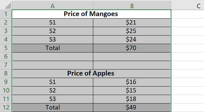
But sometimes Excel may group incorrect data when grouping automatically. That’s especially when you have different levels of information, like this:
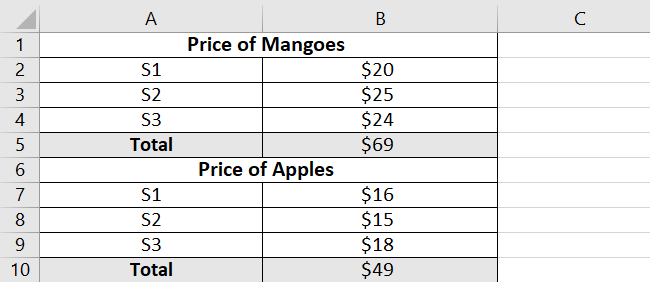
In such a case, we group the data manually.
With that being said, let’s see how to group rows in Excel both automatically and manually below.
How to automatically group rows in Excel
Suppose we have the following data that we want to group.
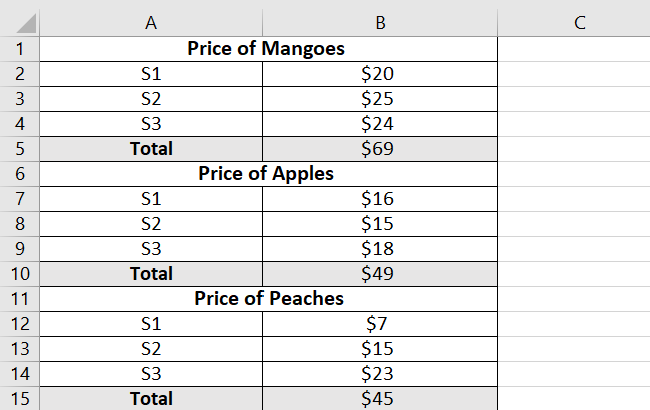
To group this data automatically:
- Select any cell from the data set.

- Go to the Data Tab.

- Under the Outline group, select Auto Outline from the Group option.

- Choose the Rows option from the Group dialog box.
- The grouped data and outline appear automatically 😉
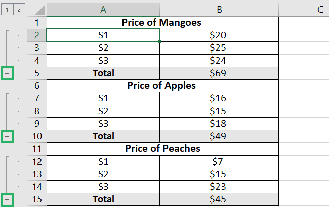
These small boxes on the left side with the minus sign are outline symbols. And they represent each level.
These boxes act like layers you can hide or show at any time to make your data more concise. It is similar to the tool used in Adobe Illustrator 🖼️
You can collapse a particular level by clicking its corresponding outline box. Like this:
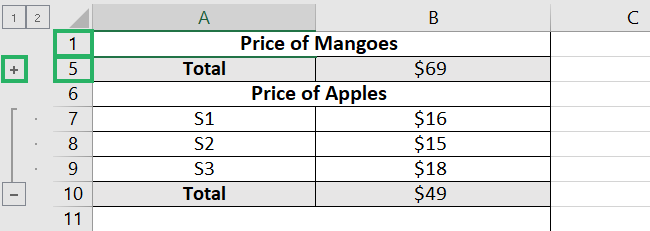
And press the plus sign to expand the rows:

We also have the outline number of each group at the top.
1 always represents the least amount of data. This is the condition where the rows are collapsed. Like this:

Similarly, number 2 represents ungrouped data.
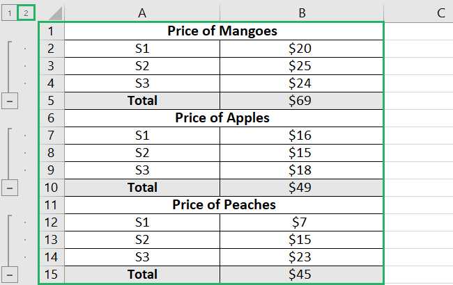
Make sure there are no hidden rows in the Excel sheet when you group data. Excel might perform the task incorrectly.
How to group rows manually in Excel
We saw earlier that Excel grouped rows automatically. But it didn’t include an outline of the whole data set. Using that outline, we would have been able to hide the entire data set.
So, how do we do that?
For that, we will group the rows manually 🔒
We will first remove the previous outline.
How to remove outlines
- Click Clear Outline from the Ungroup option under the Outline group.

- The outline disappears.

To manually group rows, we will first create the outermost outline. And then move toward the other levels.
To create the outermost outline:
- Select the whole data
- From the Data Tab, click Group under the Outline group.

- The outermost outline appears.
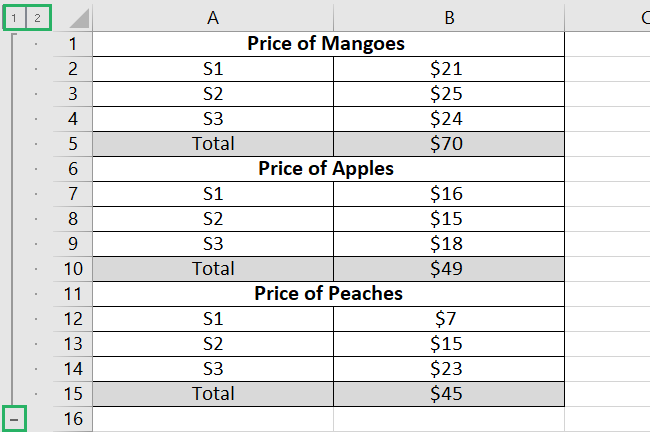
Collapsing this will hide the entire data set.
Now, for the other level, we will select a particular level each time and then group the rows together 😀
For instance, we will group the first level from A2:A4.
- Select the rows.

- Select the Group option from the Outline group.
- The selected rows have been grouped, and the outline appears.

- Perform the same steps with the remaining levels until the result looks like this.
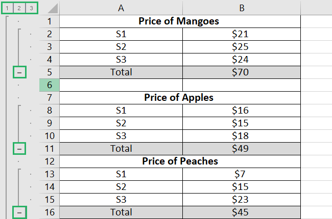
As visible, there are three number boxes in the outline this time. Contrary to what we saw earlier in automatic Excel grouping, choosing the first box here will hide all the data.
The second box will show a part of the data, and the third box will show the entire data set.
How to group rows with the SUBTOTAL function
You can also subtotal rows in all the groups using the SUBTOTAL function. You can apply the COUNT, SUM, AVG, MIN, and MAX functions to your data.
Let’s understand this with the following example data.
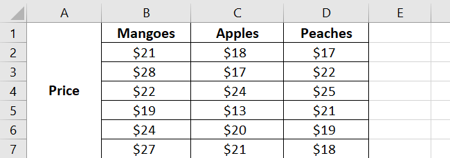
- Click anywhere on the dataset and press the Subtotal button.

- The Dialog box appears.
Select the places you want to add subtotal to.
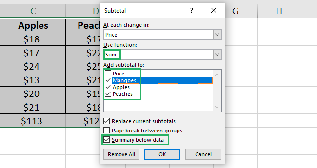
Put a checkmark on the ‘Summary below data’ option. It displays the result of the chosen function beneath the data. You can also change the function you want from the options.
The summary row looks like this:
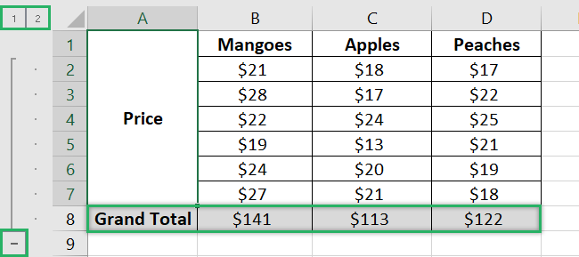
The SUBTOTAL function automatically creates an outline along with the Grand total. Hence, you can use it to get two tasks done at the same time 🤓
And that’s it about grouping rows in Excel 🤗
How to group columns in Excel
Grouping columns in excel is the same as grouping rows. It is used when your data extends from left to right instead of top to bottom.
The only difference is that the outline appears on the top of the sheet instead of appearing on its left.
Let’s see how this works.
We will use the previous data set. And here, we want to group the columns.

We will first create the outermost outline and group all the data.
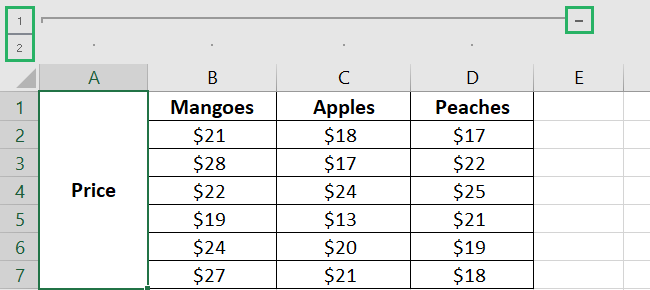
Now we will group each column individually, starting from column B – Mangoes.
- Select the column heading and click Group.
- Choose the Column option from the dialog box.
- Press Enter
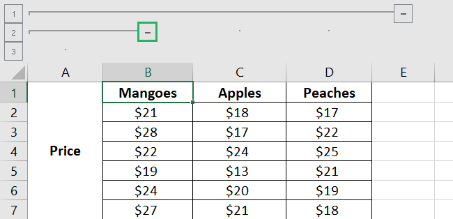
- Repeat the same process with the remaining columns.
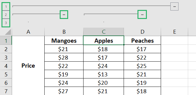
All your columns have now been grouped.
That’s it – Now what?
Knowing how to group rows or columns is very important. It helps organize data and improves the readability of complex and detailed information.
In this article, we learned how to group data in Excel and how to make a clear outline. These are some of the most useful features of Excel, but there’s so much more to learn.
If you are new to this giant spreadsheet software, we suggest you start by mastering the essential intermediate functions. These include VLOOKUP, IF, and SUMIF functions.
Join my 30-minute free email course to learn these fantastic functions and many more.
Other resources
The best part about grouping rows and columns in Excel is that it lets you focus on a small section of data instead of the whole sheet.
If you like this article, you might want to read some other articles like the SUBTOTAL function, FILTER function, or hiding rows. 😃
