How to Unhide All Hidden Rows & Columns in Excel (At Once)
Got a spreadsheet with some hidden rows?
And you don’t want to spend too much time identifying them so you can unhide them?🔍
No worries!
This guide shows you exactly how to unhide rows (and columns) in Excel in just a few minutes.
Please download my sample data workbook here if you want to tag along.
Table of Contents
Unhide all rows in Excel
Identifying hidden rows requires you to look very carefully at all the row numbers.
This is cumbersome⏳
So you definitely want to use one of several techniques to unhide all rows at once.
1. Select the rows where you think there are hidden rows in between.
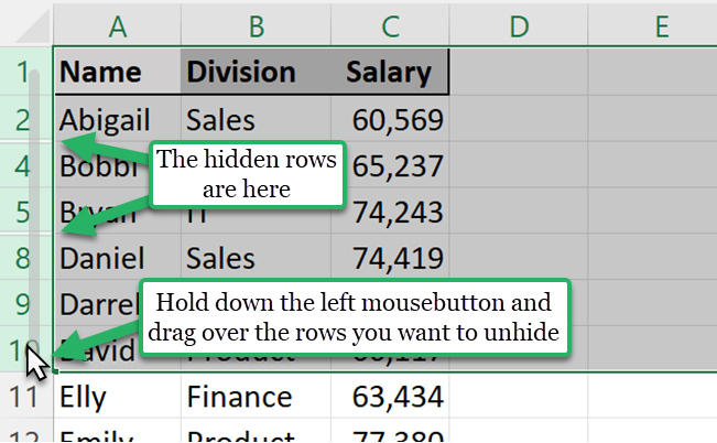
Since you can’t select the specific hidden rows, you need to drag “over” them with your cursor while holding down the left mouse button.
2. Right-click any of the selected rows.
3. Click Unhide.
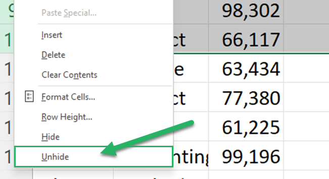
That’s it – now all the hidden rows in between the rows you selected are visible💡
Unhide rows with shortcut
Unhiding rows can be done even faster than this!
After selecting the rows in step 1 above, you can use a shortcut to unhide rows instead of doing step 2 and 3.
So, select the rows and press Ctrl + Shift + 9.
Easy, huh?
Unhide rows hidden by autofilter
Sometimes rows are hidden because of another method: the autofilter.
With the autofilter, you can easily control which rows are visible (and which are hidden).
To unhide rows hidden by the autofilter, you don’t need to jump through all the hoops.
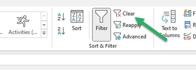
Simply go to the Data tab, and click the Clear button.
Unhide individual or multiple rows
Sometimes, you don’t want to unhide all rows, but just a specific row, or several specific rows.
To unhide multiple rows, use the same method as before:
1. Select the cell above the hidden rows, hold down your left mouse button and drag over the hidden rows – selecting them and the row below the hidden rows.
2. Right-click any of the 2 visible selected rows.
3. Click Unhide.
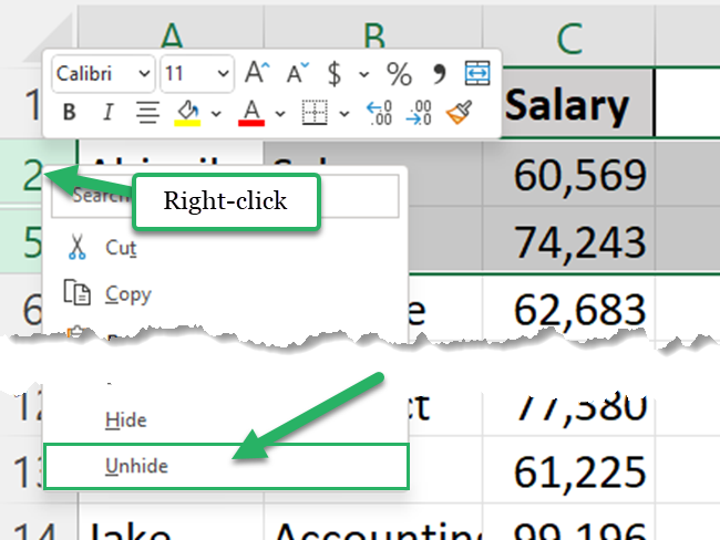
And voila! The rows are visible👓
Unhide first row in Excel
Unhiding the first row can be particularly tricky – if you don’t know how.
Because, how can you select it if you can’t “drag over” it, like with other hidden rows?
Luckily, there’s another way to select that first hidden row.
1. To the left of the formula bar there’s a name box. Write “A1” in it.

Now, cell A1 is selected.
2. On the right side of the Home tab, click Format.
3. Hover the cursor over ‘Hide & Unhide’ and click ‘Unhide Rows’.
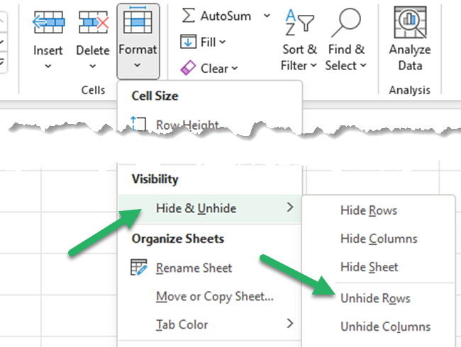
Now, the first row is visible again 👍
PRO TIP:
If you find the above method for unhiding the first row a bit too cumbersome, try this instead.
You can actually select the hidden first row by holding down the left mouse button and “dragging over” it.
You just need to start dragging from row 2 and then drag in an upwards motion that ends on row 0 (the grey triangle).

After that, just right-click row 2 and click Unhide.
Note: it’s not enough to just select row 2. You need to drag over row 1.
Unhide columns in Excel
Hidden columns can be almost as cumbersome to identify as rows.
I’ve sung the alphabet song to myself countless times to try and identify which letters (column names) were missing.
Here’s how to do it without singing🎶
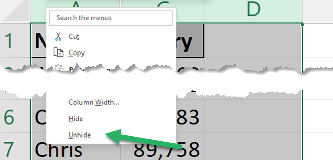
1. Select the columns where you believe columns are hidden in between. You do that by “dragging over” them while holding down the left mouse button.

2. Right-click any of the visible selected columns.
3. Click Unhide.
Unhide all rows and columns
This is your one-stop solution for unhiding all the rows and columns in your spreadsheet.
You don’t have to look for anything or spend a second thinking if you “dragged over” all the rows that could have a hidden row in between.
Here’s how to unhide all the hidden rows and all the hidden columns in one fell swoop.
1. Select all the cells in the spreadsheet by clicking the ‘Select All’ button.
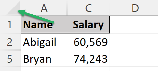
Or you can use the Ctrl + A shortcut.
2. Right-click any of the selected rows and click Unhide.
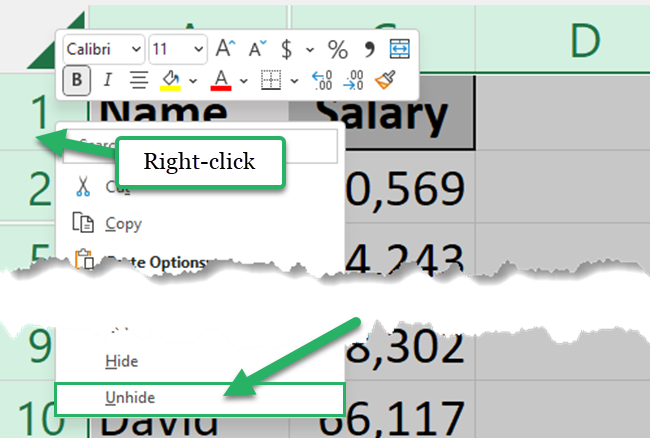
This unhides all the hidden rows.
3. Right-click any of the selected columns and click Unhide.
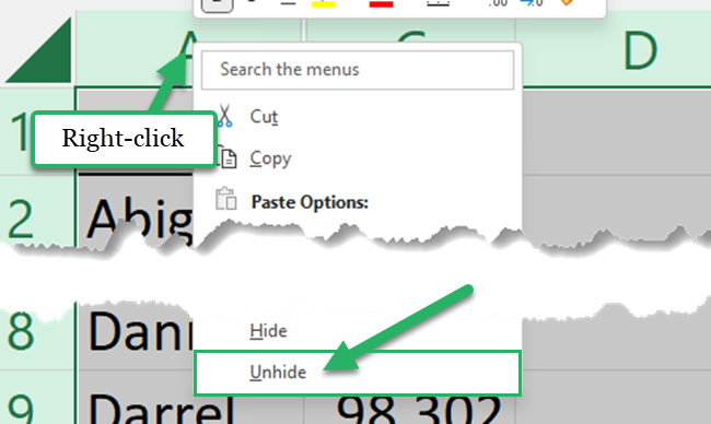
This unhides all the columns.
And that’s how you unhide all rows and columns at once🔍
VIDEO: Unhide rows and columns
More into video than text?
Watch my video and learn everything you need to know about unhiding rows and columns in Excel.
That’s it – Now what?
You just learned how to unhide all rows in Excel.
And a lot more, actually!
It wasn’t so scary after all, was it?😎
You’re unhiding rows because you want to work with the full data set, instead of just the visible part of it.
So, now that your hidden rows are visible, you should consider learning a few methods to work professionally with your data.
No matter your current skill level, I got you covered.
Click here and enroll in my free 30-minute online training.
I’ll send it directly to your inbox within 5 minutes.
Other resources
If you’ve made hidden rows visible but didn’t mean to, you can simply undo your actions with the Undo feature.
Or you can hide rows to make the data set the same as it was before.
Also, as I mentioned before, filters are a great way to work better with big data sets by hiding rows you don’t want to look at.
Make sure to learn how to unhide sheets as well!
FAQ
Got any specific questions about unhiding rows?
Read below and you may find your answer😊
