How to Paste Horizontal Data Vertically in Excel (Easy)

This tutorial is going to discuss some interesting methods to flip data in Excel.

Fun Fact: The data remains the same, and any underlying formulas also remain the same. It is just that data sorted in a horizontal shape takes a vertical shape.

In other words, you could see, rows become columns. Flipping data such that horizontal arrangements turn vertical (and vice versa) is called transposing data 🙈

And you can do it by simply copying and pasting data.

Excited to learn how to do it in Excel? Get your free practice workbook now and read with me till the end.

Paste Horizontal Data vertically by using the Transpose feature

You’ll thoroughly enjoy the process of picking data and turning it 180 degrees around without anything moving out of order.

Let me show you how to do it here 🧐

The data in the image below shows some students, their heights, weights, and ages.

Right now, it is arranged horizontally.

To copy and paste this data vertically, follow the steps below

Step 1) Select the data.

Step 2) Copy it by pressing the Control key + C.

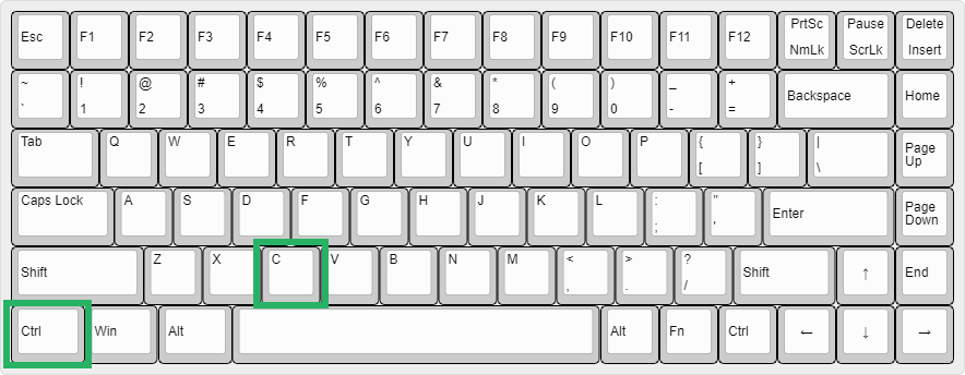
Once copied, a dotted green border will appear around the dataset.

Step 3) Select the destination cell starting from where (downwards and rightwards) you want the data placed.

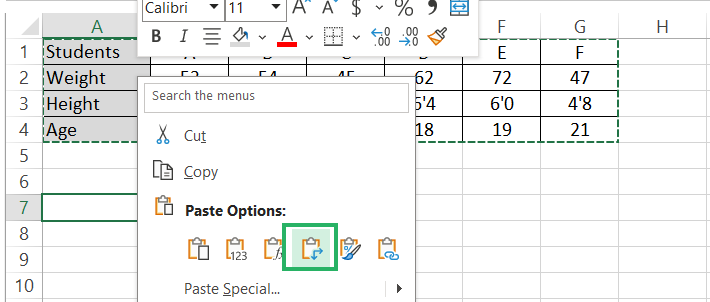
Step 4) Right-click on this cell to launch the drop-down menu of options.

Step 5) From the Paste options, select the Transpose icon.

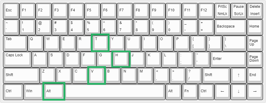
Alternatively, you can use the keyboard shortcut of the Alt key > H > V > T (pressed in a sequential order).

Kasper Langmann, co-founder of Spreadsheeto

The data will be transposed from horizontal to vertical orientation.

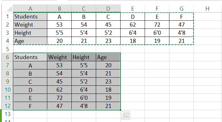
See how the formatting of the original data is copied and pasted as it is. It is this simple to flip your data vertically (or vice versa) in Excel ✌

Flip Horizontal Data Vertically using the TRANSPOSE function

Besides copying and pasting, you can also flip data in Excel using the TRANSPOSE function.

The TRANSPOSE function is an array function that returns the result as an array.

Kasper Langmann, co-founder of Spreadsheeto

Continuing with the same data as above, follow these steps to flip it around using the TRANSPOSE function 💡

Step 1) Begin writing the TRANSPOSE function.

Click to copy

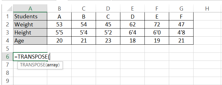
Step 2) Supply the array to be transposed as the first and only argument.

Click to copy

Step 3) Press Enter.

Pro Tip!

Since the TRANSPOSE function is a dynamic array function, if you’re subscribed to Excel 365 or 2021, pressing the Enter key alone does fine.

But if you’re subscribed to Excel 2019 or older versions, you need to press the combination of Control key + Shift + Enter for the TRANSPOSE function to work.

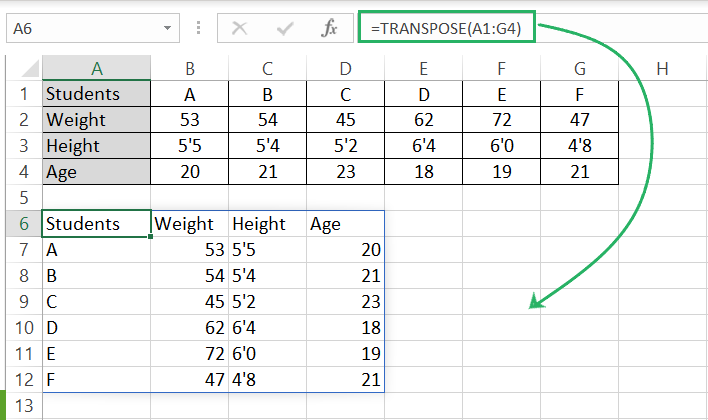
And that’s it. The data is twisted all the way around 📍

Although the TRANSPOSE function transposes the horizontal data vertically, here are some points to keep in mind while you use it:

The resulting data won’t have the formatting of the original data (see the transposed data misses out on the grey headers from the source data + the alignment of data is not the same as the source data).
The resulting array has a formula running behind. So, if you make any changes to the source data, this data will be automatically updated.
If you delete the original data from the sheet, the transposed data will also be deleted from the sheet (unless you have copied and pasted it as values).
You cannot make any changes to any individual cell of the resulting array.
Any single cell cannot be deleted from the resulting array. You can select and delete the whole array only.
If the cells needed to populate the resulting array are not empty, the TRANSPOSE function will return a #SPILL! Error.

Considering these factors, the first method (copying and pasting) might be a preferable option if you prefer simplicity and don’t want to retain both source data in your sheet once it is transposed.

In the end, you have learned both the amazing methods to flip data in Excel. Try both and see which works better for you 🤿

Conclusion

Hope you found the above tutorial not only easy but interesting.

Data positioning in Microsoft Excel can make a great difference, and if you want to make some last changes to your data to make it more readable and visually better – this guide is your savior.

Give a quick read to the following blogs too, they delve into further details of copying and pasting data in Excel to achieve different results.

Written by Kasper Langmann

Hi, I'm Kasper Langmann👋

I'm the co-founder of Spreadsheeto, a certified Microsoft Office Specialist, and a Microsoft MVP.

With over 10 years of experience, I’ve taught Excel to millions of people worldwide.

I spent over 9 hours researching and writing this tutorial.

Last updated on August 29th, 2024.

Before you go, sign up for my free Excel course (+100,000 students) ->