How to Use the IFS Function in Excel
(Many Examples)
For sure Microsoft heard you when you were struggling to construct a long nested IF function to test multiple logical criteria and brought you the IFS function instead.
Nested IF is used in Excel to evaluate situations with multiple outcomes. However, as the outcomes increase, writing this function not only becomes clumsy but time-consuming, too.
But no worries – The IFS function available in Microsoft 365, Excel 2021, and Excel 2019 substitutes nested formulas really well 🙌
In this guide, we will explore the IFS function of Microsoft Excel – from syntax to multiple practical applications. So get your free practice workbook for this guide here and stay tuned.
What is the IFS function
The IFS function in Excel is meant to test more than one criterion. If the first criteria passes the logical test; the IFS function returns the value_if_true and the formula stops.
However, if the first criteria, it then tests the next logical criteria and so on. It is designed to replace the old nested IF formula and is much easier (and simpler) to write and read 📝
Syntax
The syntax of the IFS function looks like below:
- logical_test1 is the first logical test which is a required argument and must be run.
- value_if_true1 is the value to be returned by the IFS function is the first logical test turns true. This is also a required argument.
- logical_test2 is the second logical test to be performed if the first logical test fails. It is an optional argument.
- value_if_true2 is the value to be returned by the IFS function is the second logical test turns true. It is an optional argument
Here onwards, you can specify up to 127 logical tests along with their related value_if_true to the IFS function. However, once you have specified a logical test, say logical_test3, it is mandatory to specify the value_if_true for it, or else Excel will prompt an argument that the supplied arguments are too less.
How about we now jump into seeing examples of the practical application of the IFS function?
Using the IFS function in Excel
We will now look into many examples of using the IFS function in Excel.
Let’s dive in straight 🤿
Example 1
Below is the list of members of a Hotel’s Prestige Club.
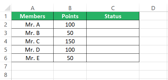
The status of these members is determined based on the number of points to their credit.
If a member has 150 points to his credit, he wins the status of a Golden member. If he has 100 points to his credit, he becomes a Golden Member and with 50 points, he stands as a Silver Member 💳
Let’s now populate the status of each member using the IFS function.
Step 1) Begin writing the IFS function as follows:
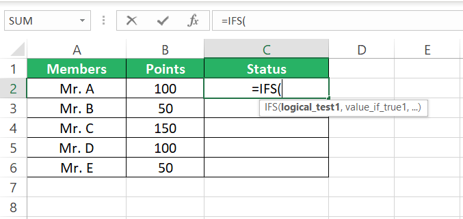
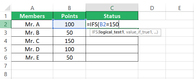
Step 2) As the first logical test, write if Cell B2 (points) equates to 150.
Step 3) Write the value_if_true as “Platinum Member”.
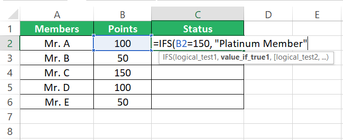
Step 4) Define the second logical test to see if Cell B2 is equal to 100.
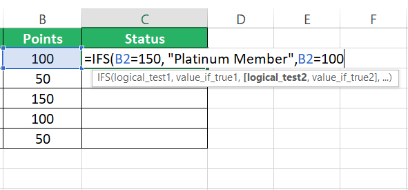
Step 5) Specify the second value_if_true as “Golden Member”.
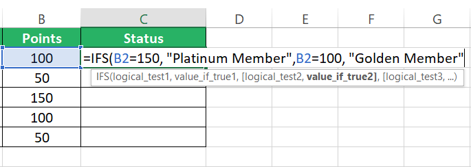
Step 6) Define the third logical test to see if Cell B2 is equal to 50.
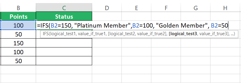
Step 7) Supply the third value_if_true as “Silver Member”.
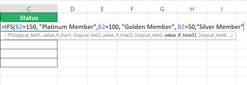
Step 8) Hit Enter to see the results.

Pretty nice. Mr. A has 100 points to his credit, so he is rightly designated as a Golden member 🥇
Step 9) Drag the results down the whole list to see the status of the other members too.

The IFS function evaluates the points of all members and returns their status as a member in a single go. Isn’t that spectacular?
Had we done the same by nesting multiple IF functions, the final function would have looked something like below 👇
Multiple nested IF statements and complex formulas. The IFS function sorts it all out.
Example 2
Time to see another and a more detailed example of the IFS function.
So here we have the scores of some students in their annual assessment, and it’s time we grade them based on their scores 🔢
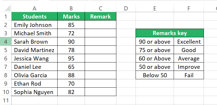
Along with these scores, we have a remarks key that tells what remark is to be assigned to each student based on his score.
Let’s begin writing then.
Step 1) Begin writing the IFS function as follows:
Step 2) As the first logical test, define the first slab of the remark key i.e., see if the score in Cell B2 is equal to or greater than 90.
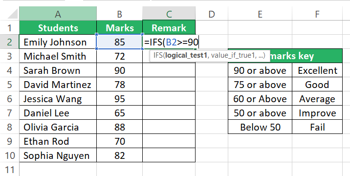
Step 3) Based on the first logical test and the remarks key, define the first value_if_true from the remarks key table.
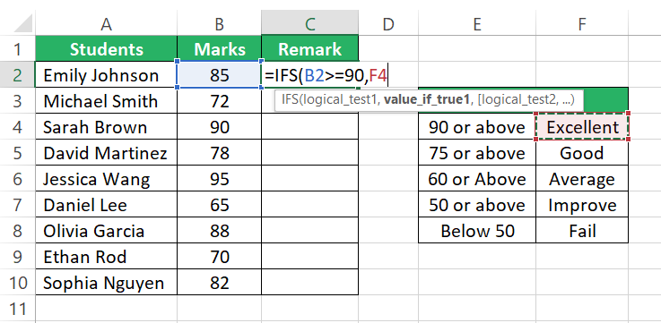
In this example, we already have the remarks defined in the remarks key table, so I am referring to the cells from the remarks instead of hardcoding the remarks in this function manually 🧾
Step 4) Define the second logical test to see if Cell B2 is equal to or greater than 75.
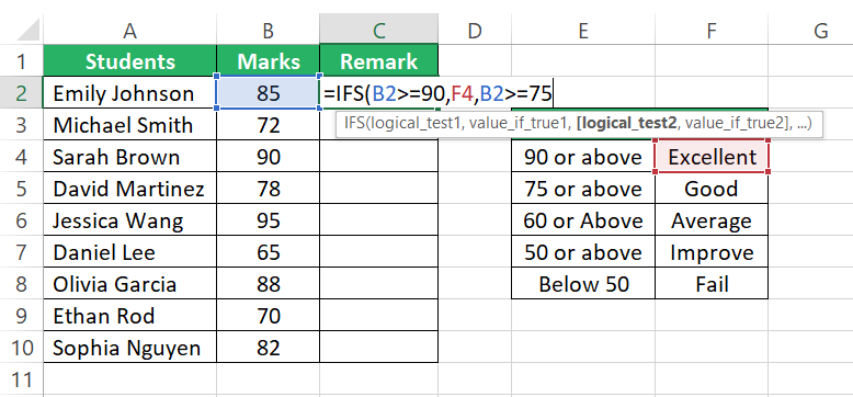
Step 5) Specify the second value_if_true as Cell F5 from the remarks key.
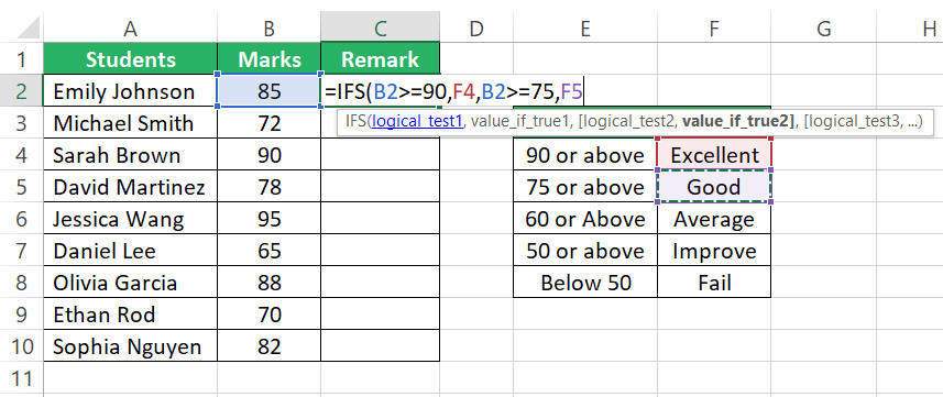
Step 6) Define the third logical test to see if Cell B2 is equal to or greater than 60 and accordingly define the value_if_true for it.
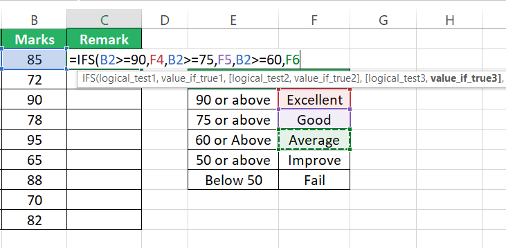
Step 7) Then comes the fourth logical test to see if Cell B2 is equal to or greater than 50 and accordingly define the value_if_true for it.
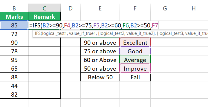
Hold tight! We are almost there 🚴♀️
All other students who scored below 50 stands “Failed”. We can specify by writing another logical test but, I will show you how to do it by manipulating it as value_if_false.
Step 8) As the next logical test, write “TRUE” or 1 and then write the value_if_false.
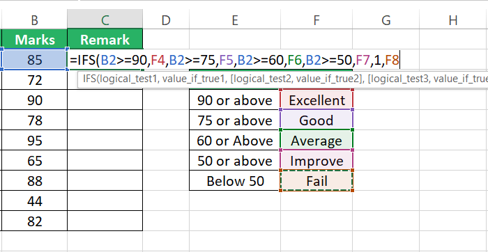
With this, our function stands completed 🎯
Step 9) Hit Enter to see the results.
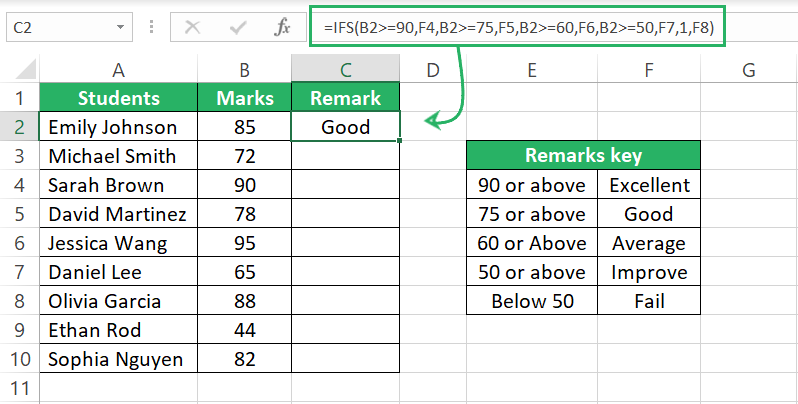
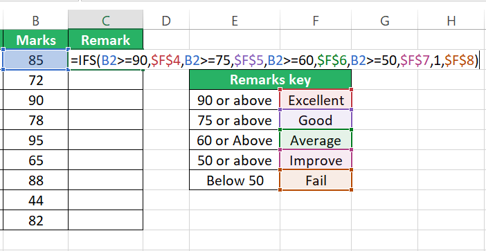
Before you drag the formula down the cells, make sure to convert the cell references for the remarks to absolute references to make sure these are not changed when the formula is dragged down.
Step 10) Drag the results down the whole list to see the remarks for all the students.
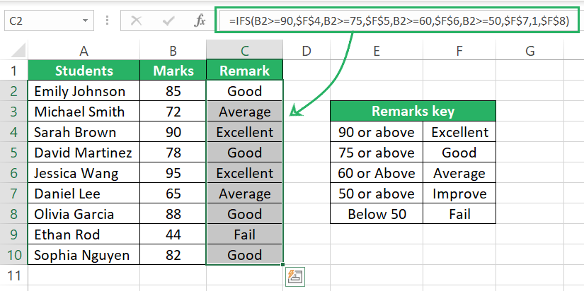
Woohoo! The entire list of scores populated like magic.
Example 3
In another example, we have some customers and the dates when their orders were shipped to them.
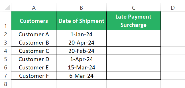
However, they have yet not made the payment against their orders. We now quickly want to run an exercise to see which customers are to be subjected to how much late payment surcharge.
If the payment of any customer is delayed by:
- More than 50 days = 10% surcharge
- More than 30 days: 5% surcharge
- More than 10 days: No surcharge
Let’s write the IFS function to automate the surcharge determination.
Step 1) Write the first logical test of the IFS function to see if the days lapsed since the order was shipped to the customer until today’s date exceed 50.
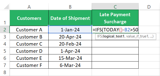
The TODAY’s function yields today’s date and deducting the order shipment date from it calculates the days lapsed in between.
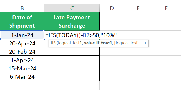
Step 2) Supply the value_if_true for the first logical test as “10%”.
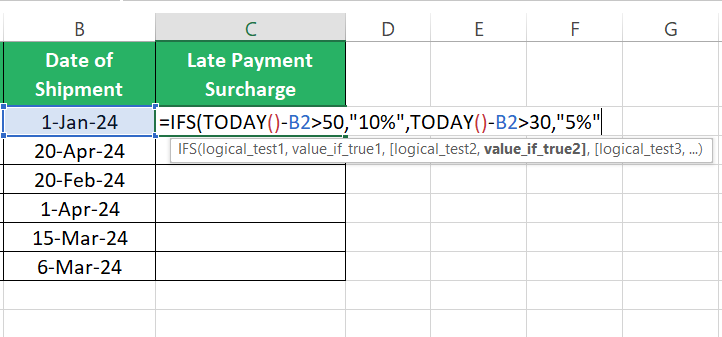
Step 3) Based on the same logic, write the second logical test to see if until today more than 30 days have lapsed since the order was shipped to the customer.
Step 4) Accordingly, hardcode the value_if_true for this logical test as “5%”.
Step 5) Then write the third and final logical test to see if until today more than 10 days have lapsed since the order was shipped to the customer.
Step 6) For this logical test, write the value_if_true as “No Surcharge”.
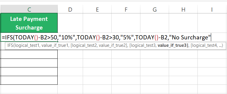
Step 7) Press enter to see the results.
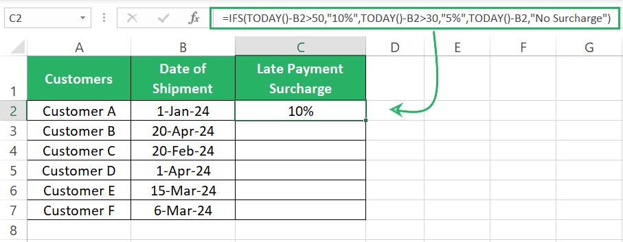
The IFS function calculates the days lapsed for each order’s shipment and based on the criteria supplied to it, determines that customer A is subject to a 10% late payment surcharge.
Step 8) Quickly drag the formula down the list to calculate the surcharge for all the customers.
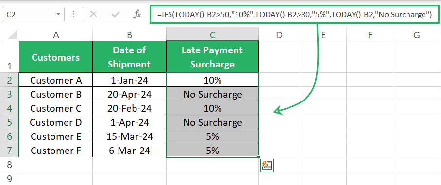
There you go! We have the late payment surcharge calculated for all the customers in a jiffy.
This example explains that even within the logical test, you can write formulas. And you can even combine functions within the logical test argument. Similarly, you can hardcode the value_if_true as a text within inverted commas or refer to other cells ⏭
Conclusion
We have seen multiple examples of using the IFS function in Excel – you must be feeling a pro at it by now. It allows users to input a series of conditions in the same function.
Be careful – sometimes the IFS function can get long and maybe, erroneous too. If you’re facing problems with the IFS function, don’t worry and read the following Excel tutorials that explain how to deal with these errors.
