How to Use Multiple Formulas in a Cell (Excel Guide)
Excel is all about smart work.
Instead of writing multiple formulas in so many cells, leveraging them together in a single cell can significantly enhance efficiency and streamline the results.
This guide provides a comprehensive overview of how to effectively integrate multiple formulas in a cell in MS Excel 😎
Through the guide, we will combine multiple functions, formulas, symbols, and text strings in a cell using an Ampersand operator (&) to produce mind-boggling results.
Download the free practice workbook for this guide here, and join us in maximizing Excel’s capabilities.
Using multiple formulas in one cell
I have a list of some items along with quantities present at a departmental store here.
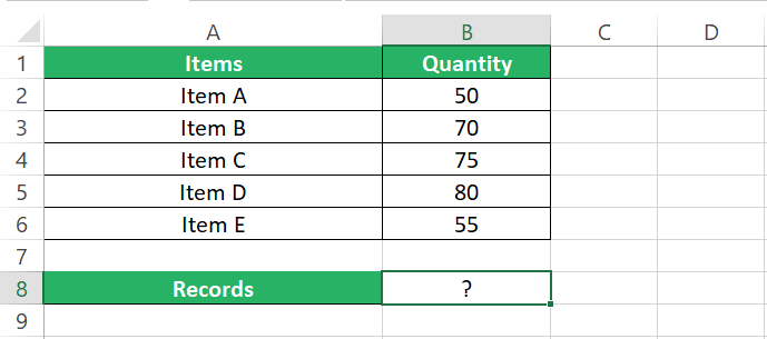
Let’s find the total items (sum of all items’ quantities) and the average quantity of each item for these items within a single cell ⚖
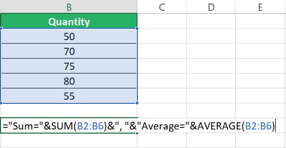
Step 1) Activate a cell and write the SUM function as below.
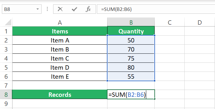
Step 2) Add an ampersand operator (&) to the above formula and add a comma in double quotation marks “,” before we write the next function

Step 3) Add another ampersand operator and write the AVERAGE function to average out the item quantities as below.
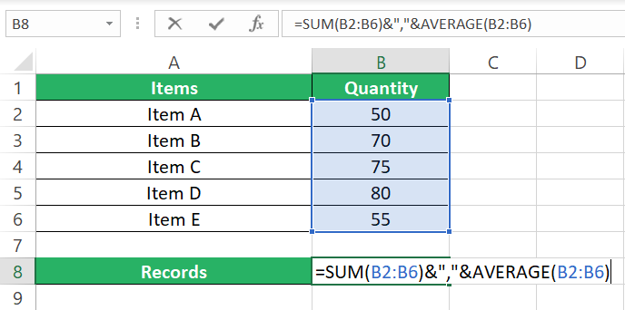
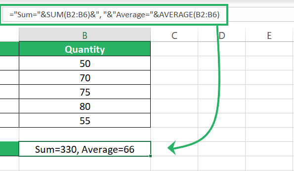
Step 4) Hit enter to see the results for this formula.
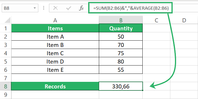
Excel calculates the sum of the quantities as 330 and the average as 66, and both results are populated in the same cell (separated by a comma) 💪
That’s how you can run multiple formulas in the same cell.
Step 5) To make it more understandable you can add the text string “sum” and “average” before both the results using ampersand.
The results look like below.
A better example of how you can combine text strings and formulas in a cell is covered in the next section 👇
Using multiple formulas and text strings in one cell
These are the marks of a couple of students from a class for three different subjects 📚
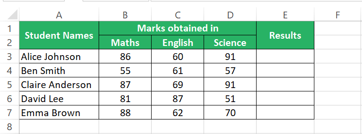
Total marks for each subject are 100, and for 3 subjects, the total marks are 300.
I want to prepare the results for all of them by calculating the total marks they have scored along with the percentage marks.
Let’s tell Excel to do it for us within a single cell in a single go using the ampersand operator (&).
Step 1) Begin writing the following formula with an equal sign:
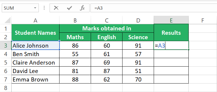
A3 contains the name of the student.
Step 2) Add an ampersand to it.
Step 3) Add another text string “ scored “. Note the [start-highlight]space character[end-highlight] I have added before and after the word within the double quotation marks.
Step 4) Add another ampersand to connect “ scored “ with the SUM function.
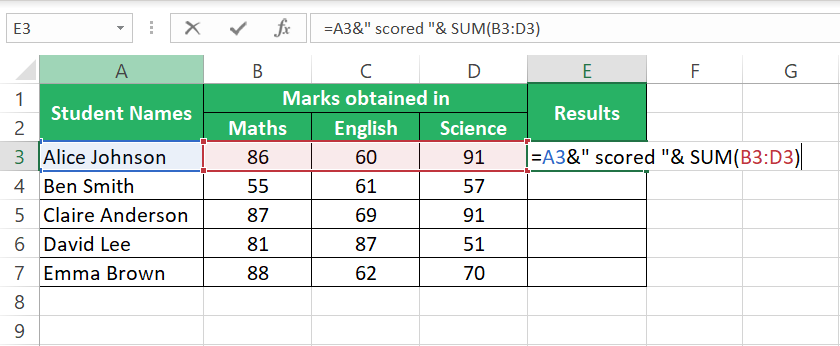
The SUM function adds up all the marks scored in each of the three subjects.
Step 5) Press enter already to see how Excel calculates the total marks, puts them in a text string, and returns it.
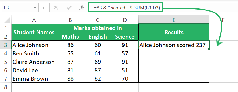
Step 6) Add another ampersand to it and connect it with the text string “ points out of 300 which makes“.
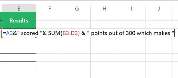
Step 7) Add another ampersand and write the formula to calculate percentage marks as:
This makes the formula look like:
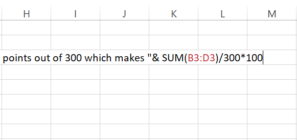
Let’s quickly hit enter and see how the formula looks until now.
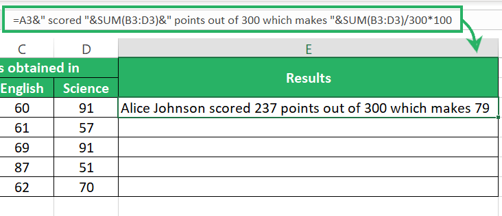
Cool. Press the F2 key to enter the editing mode again 🚀
Step 8) With an ampersand, add the percentage icon in inverted commas “% marks”. This will come next to the percentage calculated by Excel.
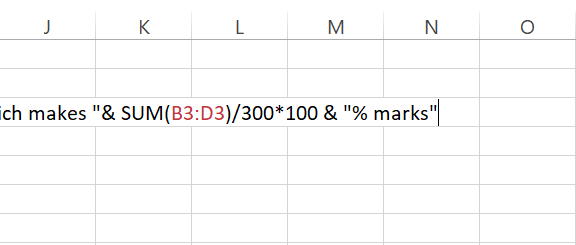
Looks long enough.
It’s time we see the results. Hold on tight, the results will have you amazed.
Step 9) Press enter to see how Excel combines all these formulas and text strings to give us a one-liner wholesome result.
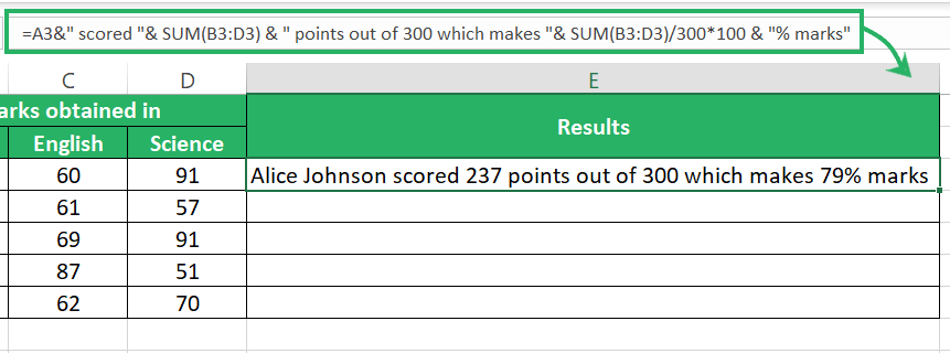
Wow! Gives such auto-generated feels ✌
The most thrilling and the best part is yet to come. Once you have put in all your brain to compose this stellar formula, you can have it ready for any number of students in a blink.
Step 10) Drag and drop the formula using the Fill handle to have the results of all students.
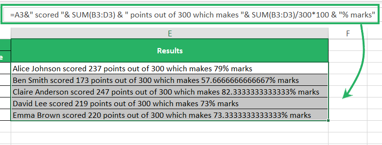
For each of the students, Excel calculates the total marks scored by them + the percentage marks secured by them.
And not merely numbers, but we have the results fixed in a proper sentence 📝
Rest assured, but some percentages look weird due to the recurring decimal positions. We cannot adjust it by formatting the decimal places to a lesser number since there are multiple formulas in this cell.
However, we can use the ROUND function to help it.
Step 11) Nest the percentage formula into the ROUND function and set the decimal places to 2.

Step 12) Now drag and drop the results to the whole list to have the percentage decimals limited to two places.

Conclusion
This guide comprehensively covers the step-by-step procedure of combining multiple formulas, functions, and text strings in a single cell.
Smartly using the above method, you can automate most of your work in Microsoft Excel in no time. There are endless variations to how can you use the ampersand operator and merge results for your good 👌
Enjoyed reading this tutorial? I suggest you read my following Excel guides, too:
