How to Change Negative Numbers to Positive in Excel

Got your data cluttered with negative numbers?

It is quite common if you’re importing data in Excel from an external source (web, a CSV file, etc.) or even if you merged data from some sources.

Unwanted negative numbers in your Excel sheet can be a nuisance, and this tutorial is meant to help it. We are going to discuss all the methods out there to change negative numbers to positive in Excel in a blink 👀

Here’s your free practice workbook for this guide, download it now and continue reading to uncover them all.

Table of Contents

Multiply with a negative number (-1)

Remember that mantra from school, “Two negatives make one positive”?

This section will show you the practical application of it 👩‍🏫

-3 into -1 makes +3 (when two numbers are multiplied, their signs are also multiplied, and two minus signs make one plus sign).

Just like this, I have a list of negative numbers here in Excel.

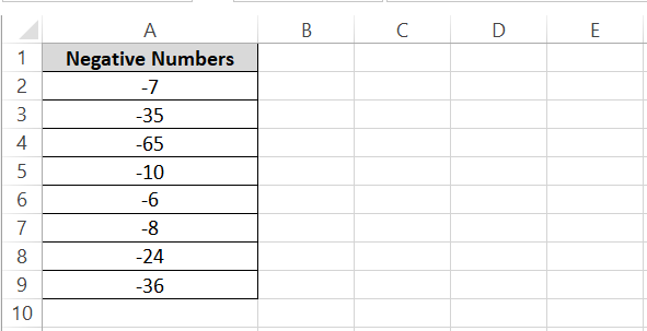
To convert these numbers to positive:

Step 1) Activate a cell from the column next to these numbers.

Step 2) Write the following formula in it:

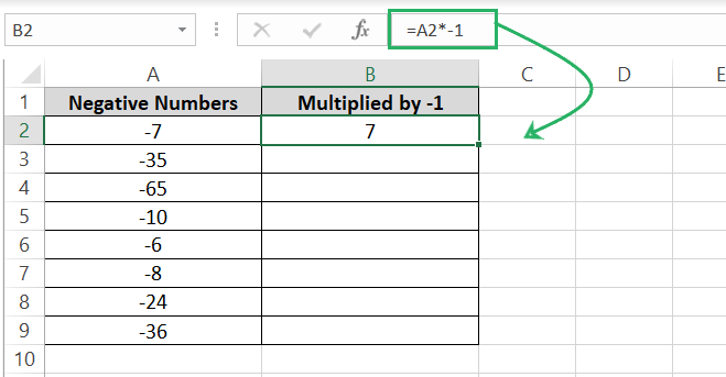
Excel multiplies the referred cell with –1, and the number turns positive 😲

Step 3) Drag this formula down the list to have the same applied to all negative numbers.

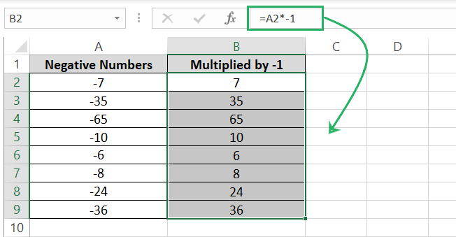
There you go!

This method creates a separate list of positive numbers (in addition to the negative numbers).

You can copy this list, and paste it as values from the Paste Special options.

Step 4) Select the column containing the negative values.

Step 5) Press the Control key + C to copy the same.

Step 6) Go to the destination cell (where you want the positive values to appear).

Step 7) Press the Shift key + F10.

Step 8) Press the V key.

Step 9) Press Enter.

Excel will paste these as values (the formula of multiplication will be replaced by the result).

Pro Tip!

Make sure your list has all negative values to use this method. If it has a mix of positive and negative values, it might distort the results.

For example, suppose the list of numbers has some positive values in between. As you drag the formula down and multiply it with -1, the already positive numbers will turn negative (a positive value multiplied by -1 makes a negative value).

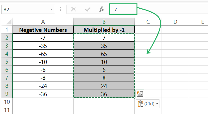
Using the Paste Special Feature

The concept remains the same (we will multiply negative values with another negative to convert it into a positive value).

However, this time, without creating an additional column 🚴‍♀️

To use the Paste Special feature to convert negatives to positives, follow the steps below.

Step 1) Activate a cell and type in -1.

Step 2) Copy this cell.

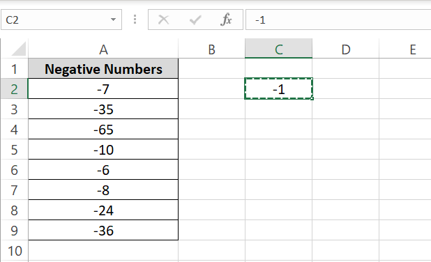
Step 3) Select the list of negative numbers.

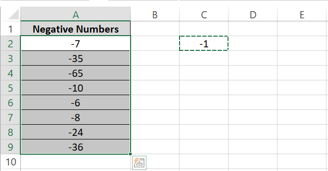
Step 4) Press the Alt Key > E > S.

This will launch the Paste Special dialog box.

Step 5) Select the option ‘Values’ and ‘Multiply’ from the Paste Special box as shown below.

Pro Tip!

You can perform both the above steps by using the shortcut keys: Alt key > E > S > V > M in a sequential order.

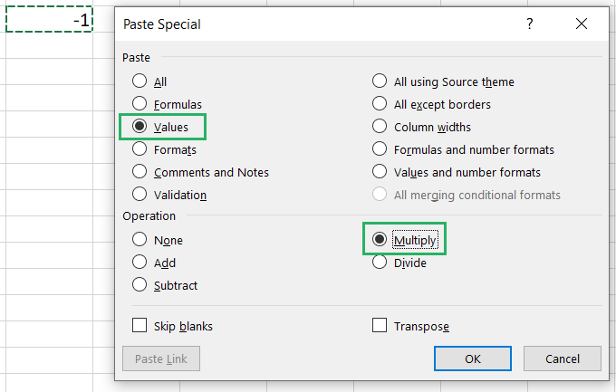
Step 6) Press Enter.

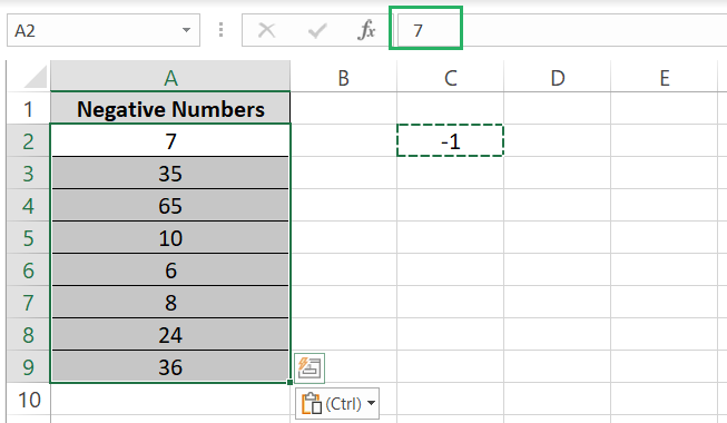
Excel copied -1 and pasted it to the negative values by multiplying.

Cool enough ⌨

Using the Flash Fill feature

The Flash Fill feature of Excel is smarter than you think and comes in handy to convert negative numbers to positive ones.

Let’s try and see here.

Step 1) Activate a cell next to the list of negative values.

Step 2) Write the first value of the list in this cell skipping out the minus sign from it.

I have written -7 as 7 in Cell B2 🏓

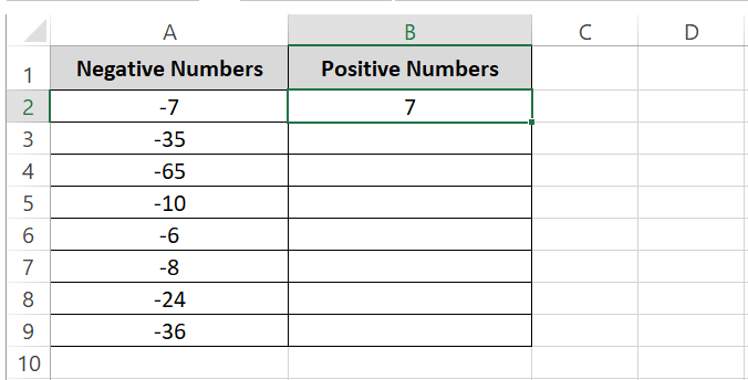
This tells Excel how to populate this column (by taking the value in Cell A2 and removing the minus sign before it).

Step 3) Select Column B up to the cell where the adjacent list of negative values goes.

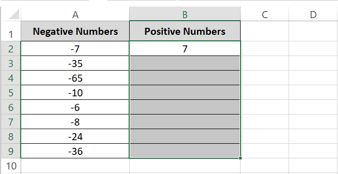
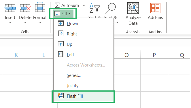
Step 4) Go to the Home tab > Editing group > Fill button > Flash Fill.

Excel will flash-fill the remaining cells based on the pattern indicated above (same value as in Column A but minus sign removed), and here are the results 🗝

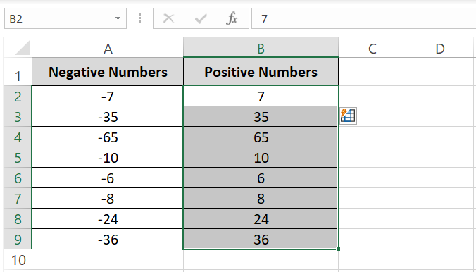
This method is quick and will work fine even if the original list of negative values contains some positive values, too.

Like here.

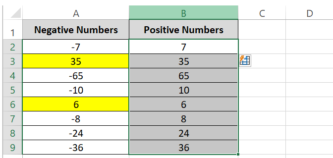
The positive values remain positive in Column B as well when the flash-fill is applied.

Using the ABS Function

ABS stands for Absolute. The ABS function is designed to turn any number into an absolute (positive) number.

Like the Flash-fill method, this method can also be carefreely applied to a list of mixed negative and positive values. The ABS function will convert any value that comes to it (whether positive or negative) into a positive number.

Let’s see it in action 🚀

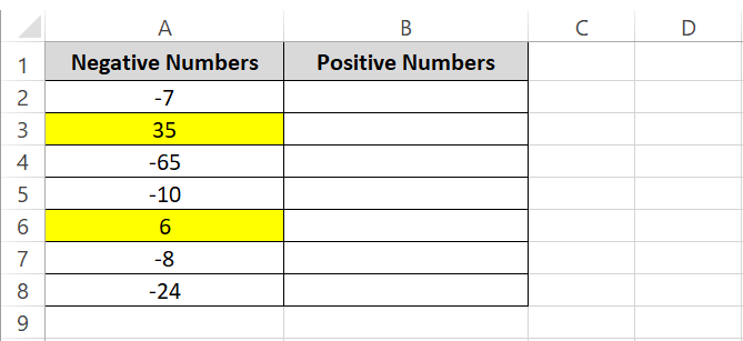
To convert all these values into positive numbers:

Step 1) Write the ABS function as follows:

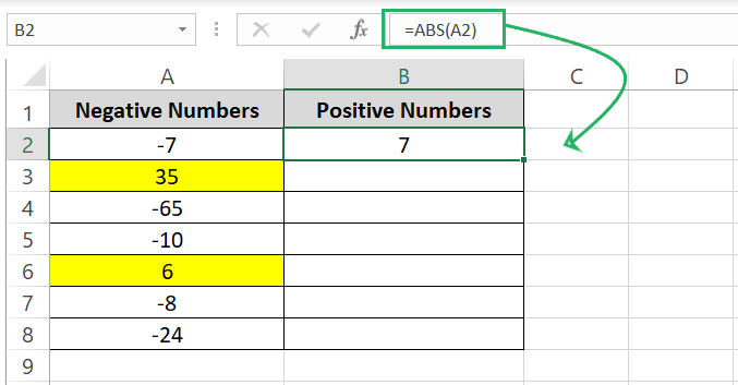
Step 2) Drag the fill handle to apply the formula to the whole list.

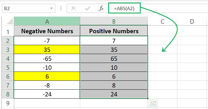
All values turn into positive numbers. And the values that were already positive remain the same 🏳

Find and Replace

There’s barely an Excel user out there who hasn’t used the Find & Replace tool of Excel.

But you can use it to convert negative numbers into positive too, this might be news to you 📝

How? Let’s see here.

Step 1) Select the cells containing the negative values.

You can skip this step if the entire sheet contains negative values that you want to be converted to positive values.

Step 2) Press the Control key + H to launch the Find and Replaced dialog box.

Step 3) Against the Find What box, write a minus sign “-“.

Step 4) Leave the Replace with box vacant as we want the minus sign replaced with nothing.

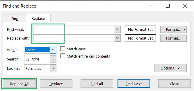
Step 5) Press Okay.

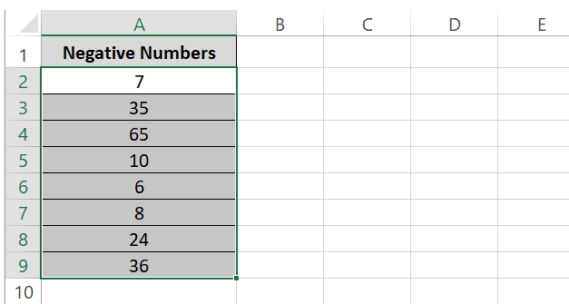
All those values with a negative sign are replaced with positive values (the minus sign preceding them has been removed leaving them positive) 💲

Other ways how you can change negative numbers to positive

We’ve already discussed the main and go-to methods to convert negative numbers into positive ones in Excel.

However, there is another way that you can explore and see if it works for you.

Custom formatting

Some of the times, the main purpose is not to convert negative numbers to positive ones but to show them as positive.

Is it possible that a number in essence stays negative but appears positive on the face of Excel?

Yes, you can format it to appear so 🏸

Step 1) Select the cells containing negative values that you want to be shown as positive values.

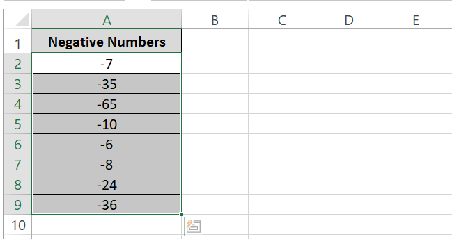
Step 2) Go to the Home tab > Number group > Number formats.

This will launch the Number Format dialog box as below.

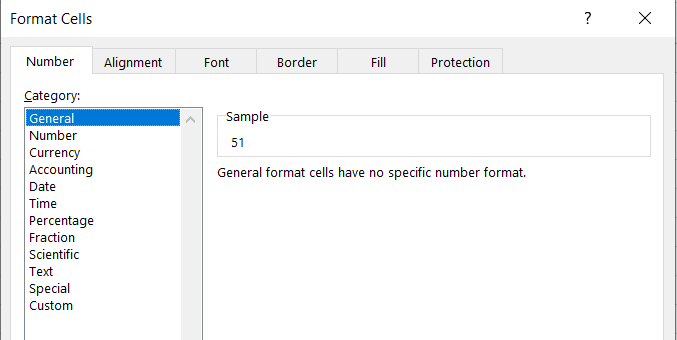
Step 3) From the pane on the left, select Custom Format.

Step 4) In the type box, type the number format as

Pro Tip!

This custom format takes four types of data formats, each of which is separated by a semi-colon.

• Positive number format (denoted by the first zero). Excel will present positive numbers as it is.
• Negative number format (denoted by the second zero). Normally it is written as -0 which, tells Excel to format all negative numbers with a preceding minus sign. We have changed it to a simple zero (without a minus sign). This tells Excel to present all negative numbers without any minus sign before them.
• Zero values.
• Text format (denoted by @ sign after the third semi-colon)

You can change the format for any of these data types here. For example, if you altogether omit the negative number format, all negative numbers will vanish from the face of your sheet.

Similarly, you can give the positive number format as +0 to have a + sign appearing before all positive numbers in your sheet.

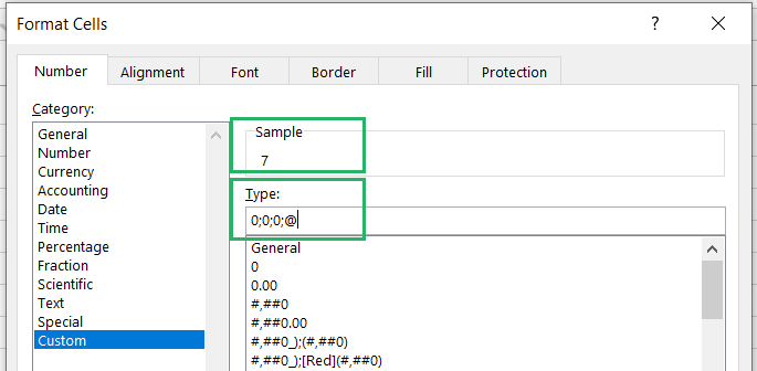
Step 5) Click the okay button to have the formatting applied.

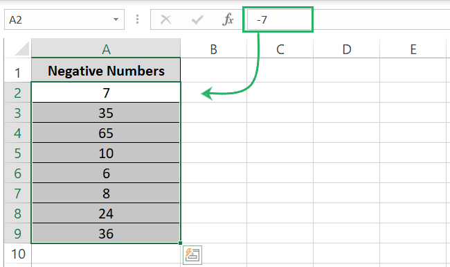
Look at the formula bar to see how only the formatting of negative numbers is changed (no more minus signs appear before them). But the negative values are still the same.

For a test and trial, let me put this into a formula to show you that 7 is still a negative value (-7) and -7+3 is equal to -4 💡

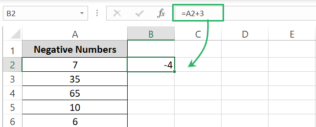
Be careful while using this method – it only helps the on-face presentation of numbers. If this is not what you desire, try other methods to change negative numbers to positive in Excel.

Conclusion

This tutorial explains all the methods to convert a set of negative (and a mix of negative and positive) numbers to positive in Excel.

You can use functions, formulas, or Excel’s smart features like Flash Fill and Find & Replace to do so. And if you’re not concerned with converting negatives to positives but only with showing them such – we still got you covered.

Read my other Excel tutorials below to learn other handy conversions in Microsoft Excel.

• The VALUE Function Explained: Convert Text to Numbers
• How to Convert Excel Formula to Value (Quickly)