How to Reference Tab & Sheet Names in Excel Formulas
Referencing the name of your sheet and tabs is a crucial skill that one needs to know to utilize Microsoft Excel to its full potential 💪
Excel allows you to store and manipulate data across multiple worksheets in your workbook easily. But how do you reference those worksheets in different places? 🤔
By using Excel formulas. These are a combination of different functions that work together to extract the tab names dynamically and reference them in cells.
We will see all of this and more in the tutorial below. But before that, download our sample workbook here so you can practice along in real-time.
Reference Tabs & Sheet Names Using TEXTAFTER Function
Let’s first see the fastest way of referencing tabs and sheets in Excel if you quickly want to have the solution or have the new version of Excel 😁
The TEXTAFTER function is the latest Excel data manipulation function that returns text after a certain delimiter. Currently, it is only available in Microsoft Excel 365.
If you do not have MS Excel 365, try other methods below – they are just as easy but slightly longer. But don’t you worry, we will guide you through everything 😀
We have the following five sheets in our Excel workbook – one of which is Summary. In the Summary sheet, I want to write down the names of all my worksheets dynamically.

We will use a combination of CELL – which returns the location of a cell and TEXTAFTER function – which returns the text. Their syntaxes are given below:
where,
info_type refers to the type of information you want to extract
reference refers to the cell whose location is to be extracted.
and,
where,
text refers to the text you want to extract a string from
delimiter refers to the point after which text is to be extracted
But don’t worry, we will see how to deal with this later.
First things first, we will locate the name of our worksheet.
To do that,
Step 1) Open the sheet you want to extract the name of and select a cell.
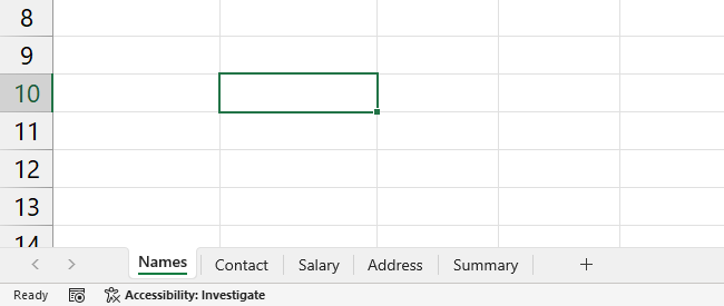
Step 2) Type in the following CELL formula in any cell
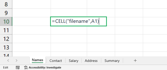
Step 3) Press Enter
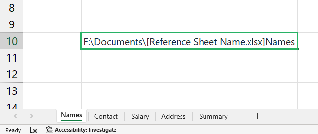
Make sure your file is saved before you apply the formula, or it will return a blank value
The CELL function returns the full path where the file is stored and the name of the worksheet we are currently in.
Now, to apply the TEXTAFTER function,
Step 4) Select a cell in the worksheet.
Step 5) Type in the following formula
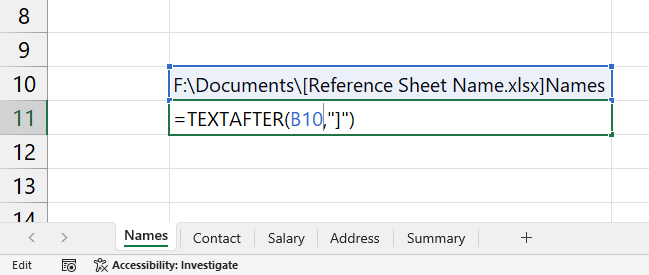
Or you can directly write the formula as ⌨
Step 6) Press Enter.
The formula will return the current sheet name as:
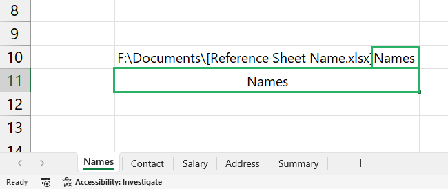
Do the same for all four sheets.
Simply copy the formula from the formula bar and paste it one by one on all sheets.
Then, list them in the Summary sheet. To do that,
Step 1) Select cell A2.
Step 2) Type = in the cell.
Step 3) Click on the tab you want to reference.
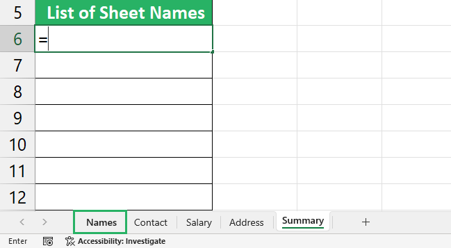
Step 4) Select the cell containing the name of the sheet.
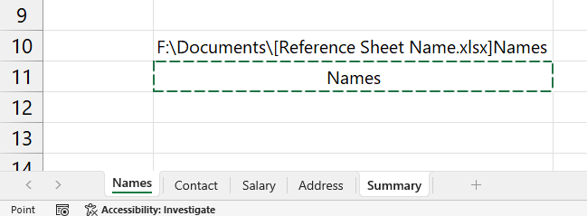
Step 5) Press Enter.
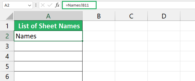
Excel returns the name of the tab in the Summary sheet. Since this formula is dynamic, the name will change here if you rename the sheet.
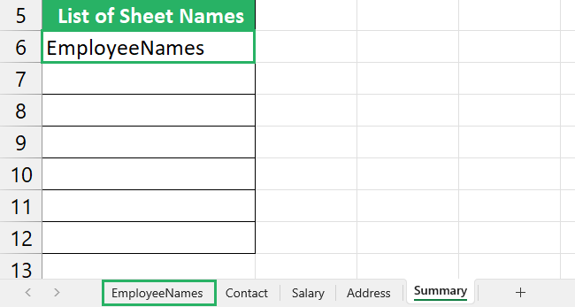
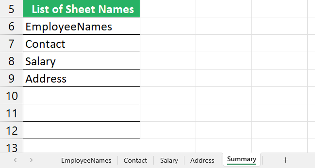
Repeat the same process for the remaining sheets and it’s done 😀
Reference Tabs & Sheet Names Using FIND Function
Let’s now see another way of finding the sheet name. It works the same as the TEXTAFTER function but is just a variation of the same for Excel users who have other Excel subscriptions.
To find tab names, we will use the combination of MID and FIND Excel functions for this method, where the MID function returns the characters at the middle of a string, and FIND locates and returns that string 🧵
The syntaxes of the two functions are given below:
where,
textrefers to the text from which the substring is to be extracted
start_num refers to the starting position of the substring – the +1 tells the function to start reading immediately after the character criteria
num_chars refers to the number of characters to read.
where,
find_text refers to the string to be found
within_text refers to the string to be found within
Let’s now implement this function below.
Step 1) Select any cell in the worksheet.
Step 2) Type in the following formula
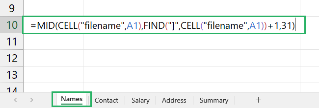
In this formula, the first argument gives the MID function the string where it has to get the sheet name, the second argument a square bracket tells the function it has to look for this and begin reading after it. The last argument is the number of characters the name of a worksheet can be, i.e. 31.
Step 3) Press Enter.
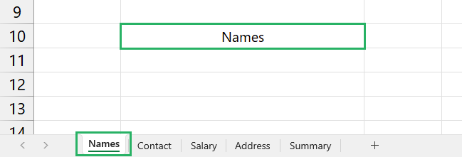
It returns the name of the active sheet , i.e. Salary.
If you were to copy this formula and paste it into another sheet to extract the name of that tab, the name in the previous sheet wouldn’t change owing to the cell reference we added.
However, if we were to skip the cell reference parameter in this formula, when we paste the formula to another sheet, its previous copy will reflect the new changes too 🧾
Paste the formula without the cell reference to the Address sheet.

Go back to the Salary sheet.
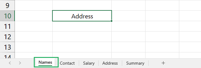
As said, the worksheet name in the previous file has now changed to that of the new one.
This error can get tricky to debug and mess up the working of your sheet if omitted accidentally. Make sure to double-check once you’re done writing the formula.
Now, following the same method as above, list all these values in the Summary sheet and you’re good to go. Try it yourself! 😃
And that wraps it up! 🎯
Reference Tabs & Sheet Names Using SEARCH Function
The SEARCH function is slightly longer than the FIND function but returns the same result. The only leverage you have here is if you have sheets of varying lengths, the LEN function here can be helpful in that 😀
It uses a combination of the RIGHT, LEN, and SEARCH functions. The syntaxes of these functions are as below:
where
text refers to the string to be extracted
num_chars refers to the number of characters to read from right
and,
where,
text is the string whose length is to be returned
and,
where,
search_text refers to the string to be searched
within_text refers to the string to be searched within
Now, to implement this function,
Step 1) Select a cell in your sheet.
Step 2) Type in the following formula
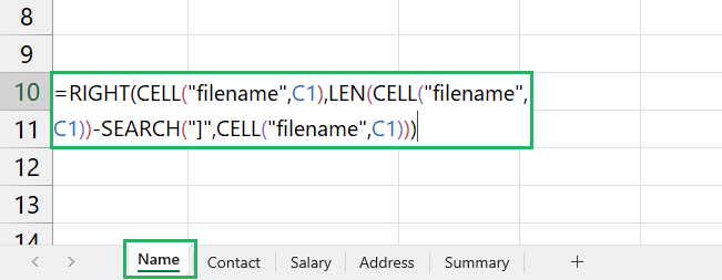
In this formula, the RIGHT function takes in the full path and places the cursor at the end. The LEN function returns the length of the path and the SEARCH function looks for the right square bracket in the string.
Once found, the length of characters before the square bracket is subtracted from the total path length and the RIGHT function then reads the sheet name from the end.
Step 3) Press Enter
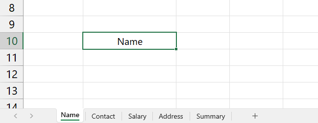
The function returns the current sheet name,i.e. Contact
The same is true if your sheet name consists of spaces or other characters.
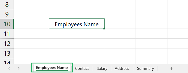
This formula can be a little tricky to get around but once you do, referencing your sheet name in Excel is going to be easy 🧐
Conclusion
In this article, we saw three different formulas that you can use to reference a tab name in your worksheet. These included the TEXTAFTER and combinations of FIND and SEARCH functions 🔍
Being able to reference tabs and sheets in formulas is an essential skill in data manipulation and is very useful if data analysis is your day-to-day task 💻
You can learn more about these functions below
Excel Functions LEFT, RIGHT, MID, and LEN for Substrings
Excel SEARCH and FIND Functions: Step-by-Step Guide (2024)
How to Rename a Sheet in Excel: Step-by-Step Guide (2024)
We hope you enjoyed reading this article as much as we enjoyed creating it.
