How to Remove Dashes in Excel: Step-by-Step Guide
Is your Excel data full of unwanted characters (more particularly dashes)? That’s just alright. You might have to face this situation every once in a while 💁♀️
Especially, if you get to import data in Excel from External sources like the web or pdf files, etc.
There are many ways how you can remove dashes in Excel. No, not manually.
I will walk you through a couple of ways to automate dash removal in Excel. So let’s not waste any more time and jump right into the guide below 👇
Table of Contents
How to remove dashes with Find and Replace
You might have guessed on this method already.
The first and easiest way to remove dashes from your Excel worksheet is by using the Find and Replace feature. Let’s do it here 🧐
The data in the image below has the names of some employees, along with their employee codes.
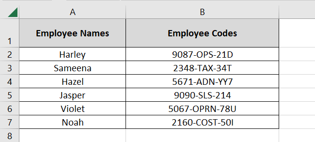
Look into the data more carefully to see the dashes in between the employee codes. Can we just get rid of them? For that:
- Select the data from where the dashes are to be removed.
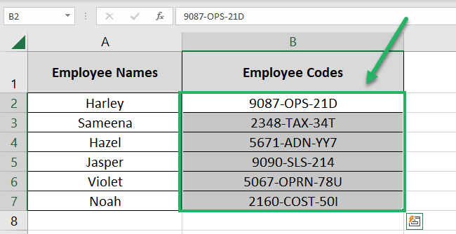
We are selecting the Cell range B2 to B7 (cells that contain the employee codes with dashes).
Do not select any data if you want to remove dashes from the whole spreadsheet ❌
- Go to the Home tab > Find & Select > Replace.
Alternatively, you may use the keyboard shortcut: Control Key + H. This will launch the Find & Replace dialog box as follows:
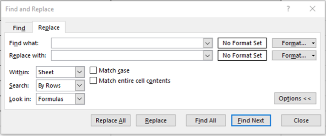
- Type in a dash against the box for Find 🔎
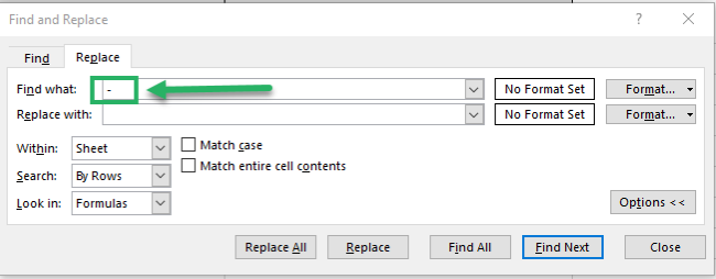
- Leave the box for Replace empty.
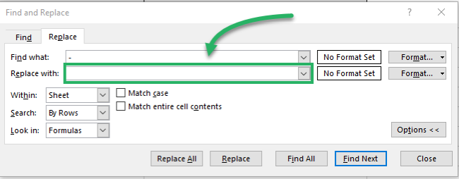
Technically, we are telling Excel to find dashes in the selected data. And then replace them with an empty string 🚀
In other words, we are telling Excel to simply remove all the dashes from the selected data.
- Click on Replace All, and there you go!
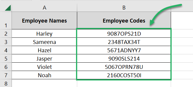
The employee codes have no more dashes to them. Isn’t that just too easy?
Remove dashes with the SUBSTITUTE function
Another convenient method to get rid of dashes in Excel is by using the SUBSTITUTE function.
Let’s remove the dashes from the employee codes in our example above using it.
Just like the name suggests, the SUBSTITUTE function substitutes (or replaces) the specified characters of any cell or text string with the new specified characters 💪
- Write the SUBSTITUTE function as follows:
= SUBSTUTTE (B2
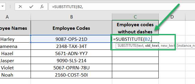
The first argument of the SUBSTITUTE function refers to the cell that contains the text to be replaced.
We want to remove dashes from the content in Cell B2 so we have created a reference to it.
- Specify the old text to be substituted. We are writing it as “-“ (dash in double quotation marks).
= SUBSTUTTE (B2, “-“,
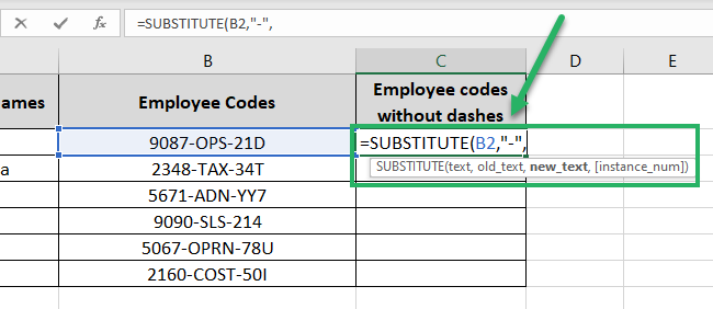
Excel will only recognize the dash (-) as text when it is enclosed in double quotation marks 💭
- Specify the new text (the text with which you want the dashes replaced).
= SUBSTUTTE (B2, “-“,””)
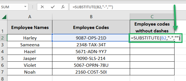
We don’t want to replace the dashes but remove them entirely. So we will enter empty double quotation marks (“”) as the new text.
- Hit Enter to get the following results.
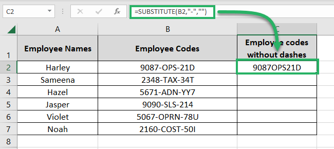
And there you go! We have the text of Cell B2 reproduced with no more dashes in between 💡
- Drag and drop the same formula to the whole list.
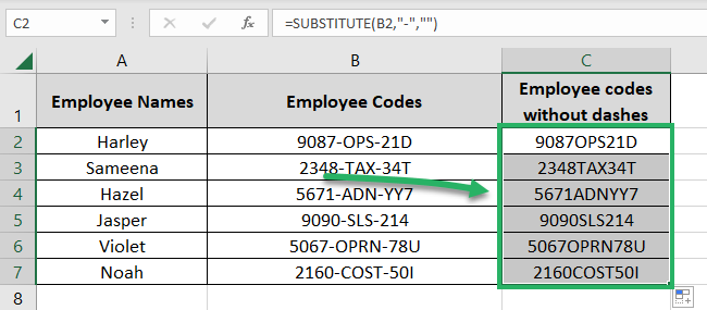
How to remove 2nd dash
Until now, we were dealing with scenarios where we wanted to remove all the dashes from our dataset.
But this scenario is somewhat different. This time, we only want to remove the second dash from each cell (not all the dashes) 2️⃣
To do that:
- Write the SUBSTITUTE function as follows:
= SUBSTUTTE (B2
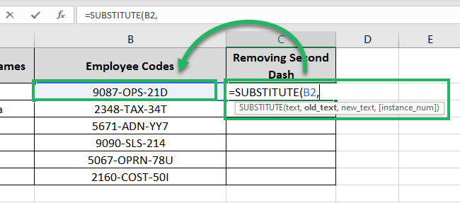
Referring to the cell that contains the text with dashes.
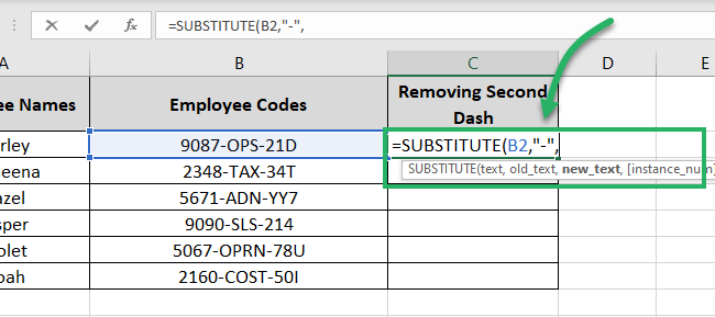
- Specify the old text to be substituted (dash in double quotation marks).
= SUBSTUTTE (B2, “-“,
- Specify the new text.
= SUBSTUTTE (B2, “-“,””,
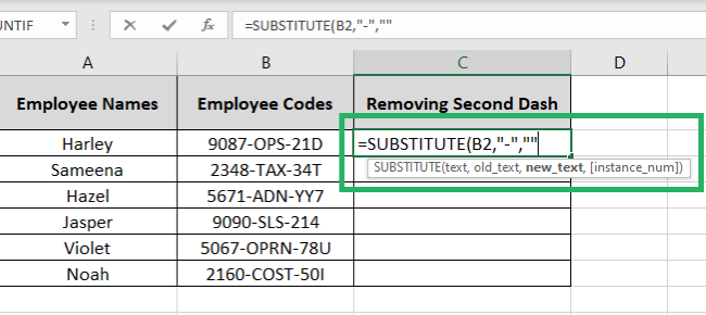
We will again set this argument to empty double quotation marks (“”) as we want the dash to be removed 🙈
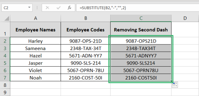
- As the instance_num argument, write 2.
= SUBSTUTTE (B2, “-“,””, 2)
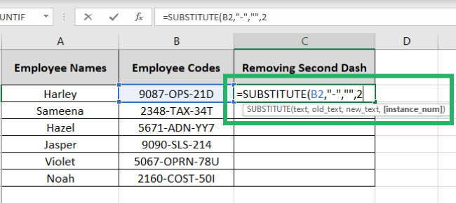
The instance number tells which instance of the old text is to be replaced with the new text.
By setting the instance number to 2, we are telling Excel to replace the second dash only.
Pro Tip!
The instance number is only an optional argument 🚫
If omitted, the SUBSTITUTE function will replace all instances of the old text in the cell with the new text. Just like we did in the above section remove all the dashes from each cell.
- Hit Enter.
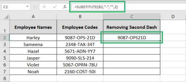
See that? Only the second dash from each employee code is removed.
- Drag and drop the same formula to the whole list.
That’s it – Now what
With these easy (and efficient) tricks, you’re all set to steer your Excel spreadsheets clear of any unwanted dashes.
Let me tell you – using these methods you can not only remove dashes but most of the other redundant characters, too. 🎯
Just like the SUBSTITUTE function, there are so many more functions of Excel that you’d love to learn about.
Like the VLOOKUP, SUMIF, and IF functions (my all-time favorite from the Excel functions library).
Want to learn them already? Click here to enroll in my 30-minute free email course that will take you through these and many more Excel functions in no time.
Other resources
Okay! So, we’ve seen how to remove dashes in Excel. But do you know how to insert dashes and other special characters in Excel?
No? Learn that here in our blog on how to insert special characters and symbols in Excel.
