How to Remove Characters From Left in Excel (Easily)

Cleaning text data from the left (or the beginning) of text strings is one of the most time-consuming tasks in Excel. 😩

However, when you know what the correct Excel formulas to use, it doesn’t have to be.

You can easily remove characters from the left of text strings in Excel to ensure better data quality and consistency. This also enhances your Excel productivity as you don’t have to manually clean up data anymore. ⚡

Learn how to remove characters from the left easily with this step-by-step Excel tutorial. Download this sample workbook and let’s start.

Table of Contents

Remove Characters from the Left using Formulas

Microsoft Excel offers a variety of functions that will help you remove characters from the left of your text strings easily and quickly.

The most commonly used Excel functions to do this are the REPLACE function and a combination of the RIGHT function and LEN function.

Remove using the REPLACE Function

Using the REPLACE function is one of the fastest ways to remove unwanted characters from the left of your text string.

As the name of its function suggests, it replaces a part of a text string based on the number of characters you specify, with a different text string or even an empty string.

The syntax of this function is =REPLACE(old_text, start_num, num_chars, new_text) with the following arguments:

• Old_text (Required) – text in which you want to replace some characters.
• Start_num (Required) – the position of the character in old_text that you want to replace with new_text.
• Num_chars (Required) – The number of characters in old_text that you want REPLACE to replace with new_text.
• New_text (Required) – The text that will replace characters in old_text.

Open your sample Excel workbook and let’s see the REPLACE function in action. 💪

Let’s say you want to clean up the original data in column A by just getting the names and removing the extra numbers on the left of the string.

To do that,

Step 1) Double click cell B2 and type =REPLACE(

Step 2) For the old_text argument, click the cell reference which contains the original data. In our example, it’s cell A2. Then type a comma symbol (,)

Step 3) For the start_num argument, type 1 for the starting position of the character in the old text that you want to replace with the new text. Then, type a comma (,)

Step 4) For the num_chars argument, type 2. This means that you’ll be replacing 2 of the number of characters in the old text. Then, type a comma symbol (,)

Step 5) For the new_text argument, type a quotation mark (““). This means you’ll be replacing the 2 first characters in the old text with an empty string. Then close the formula with a right parenthesis.

Step 6) Press Enter.

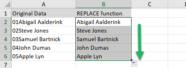
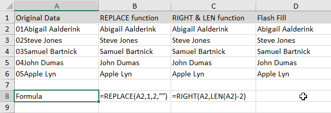
Here, the REPLACE function replaces the first 2 characters with an Empty String (“”) and results the remaining characters (name) in column B.

Fill in the rest of the rows by double-clicking or dragging down the fill handle. 👍

Remove using RIGHT and LEN functions

You can also remove a fixed number of characters from the left of your text strings using a combination of RIGHT and LEN functions. This is best used when your data set is consistent and follows the same pattern.

The RIGHT function returns the last character or characters in a text string, based on the number of characters you specify.

The syntax of this function is =RIGHT(text,[num_chars]) with the following arguments:

• Text (Required) – The text string containing the characters you want to extract.
• Num_chars (Optional) – Specifies the number of characters you want RIGHT to extract.
  • Num_chars must be greater than or equal to zero.
  • If num_chars is greater than the length of the text, RIGHT returns all of the text.
  • If num_chars is omitted, it is assumed to be 1.

On the other hand, the LEN function returns the number of characters in a text string. Simply put, the length of the string.

The syntax of this function is =LEN(text) with the following argument:

• Text (Required) – The text whose length you want to find. Spaces count as characters.

Going back to our sample worksheet, let’s remove 2 specific characters from the left of the string in each cell. 👇

Step 1) Double-click a cell and type =RIGHT(

Step 2) Click the cell which contains the text string you want to extract from. In our example, it’s cell A2. Type a comma symbol (,)

Step 3) Type the LEN function, LEN(

Step 4) Click the cell A2, then close with a right parenthesis.

Step 5) As we want to remove the first two characters from the left, type -2.

Step 6) Press Enter

The following formula uses the LEN function to get the total number of characters in the cell in column A.

From the value that we get from the LEN function, we subtract 2, as we only want to remove the 2 numbers and get the names as the result.

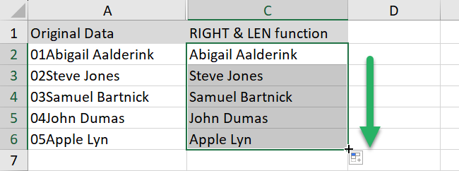
This value is then used within the RIGHT function to extract text except the first 2 characters from the left. 😊

You can fill in the rest of the rows by double-clicking or dragging down the fill handle.

Bonus: Remove Characters from the Left using Flash Fill

Another way to remove text characters from the left of a text string is Flash Fill. ⚡

You don’t need to type an Excel formula for this. You can let Microsoft Excel do it for you.

Flash Fill is one of the most amazing Excel features as it automatically fills your data when it senses a pattern.

In a separate column in our sample worksheet, let’s remove unwanted characters in the cells using Flash Fill. To do that,

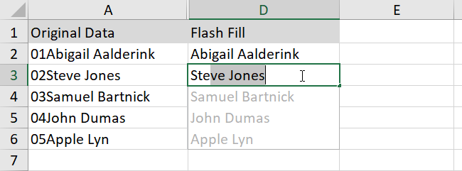
Step 1) Enter the full name in cell D2, and press ENTER.

Step 2) Start typing the next full names, Excel will sense the pattern you provide, and show you a preview of the rest of the column filled in with your combined text.

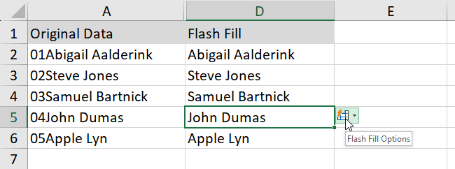
Step 3) To accept the preview, press ENTER.

Amazing, right?

This is how your sample workbook should look like.

That’s It—Now What?

Awesome! 🙌

You’ve learned 3 simple and easy ways how to remove characters from the left of text strings in cells. Now, you can clean up your data and get the results you’re after.

Want to learn more Excel formulas to help with your data and enhance your productivity? Here are our top picks:

• Excel Functions LEFT, RIGHT, MID, and LEN for Substrings
• How to Extract First Word in Excel in Less Than 1 Minute
• EXCEL TRUNCATE: Get Rid of Decimals From Numbers (+ Trim Text)
• How to Use Find and Replace in Excel: Full Guide