How to Use the Subtotal Function in Excel: Step-By-Step
We all have used the contemporary functions of Excel – the SUM Function, the AVERAGE function, the COUNT function, and so on 📝
But today, we are going to introduce you to such a versatile function of Excel that will knock your socks off. This one function can perform all these functions.
And it is no other than the SUBTOTAL function of Excel. What is it about? And what can it do? We will learn all of this in the guide below.
So continue reading and download our free sample workbook here to tag along with the guide.
Table of Contents
How to SUBTOTAL in Excel
The SUBTOTAL function can perform a range of functions on a filtered part of a list or a database.
Here’s the syntax of this function 🔍
=SUBTOTAL (function_num, ref1, ref2 … )
The Function_num
The function_num tells SUBTOTAL which function is to be performed. Here’s the list of options available to you:
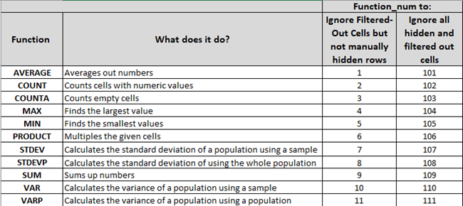
For each of these functions, there are two options.
With function number series 1-11: You can choose to include the filtered cells + any manually hidden rows in your subtotal.
With function number series 101-111: You can choose to exclude the manually hidden rows from your subtotal and include the filtered rows only.
Ref1, Ref2, and so on
These arguments refer to the values or ranges of the subtotal.
Ref1 is a mandatory argument. Ref2 and onwards the arguments are optional. And these can go up to 254 arguments.
Okay, done with the talk now. Let’s now see the SUBTOTAL function in action 🎬
Here we have a list of sales transactions for some products. And we want the sum of sales of Product A on 01 January 2022.
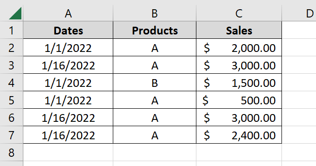
For that:
- Select the data and go to the Data tab > Filters.
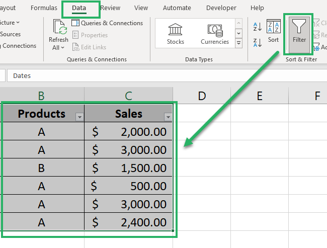
- Once you have the filters applied to your data, click on the filter icon on Dates to filter out the sales for 01 Jan 2022.
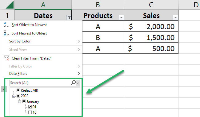
- Filter out the sales of Product A by clicking on the filter icon on the header “Products”.
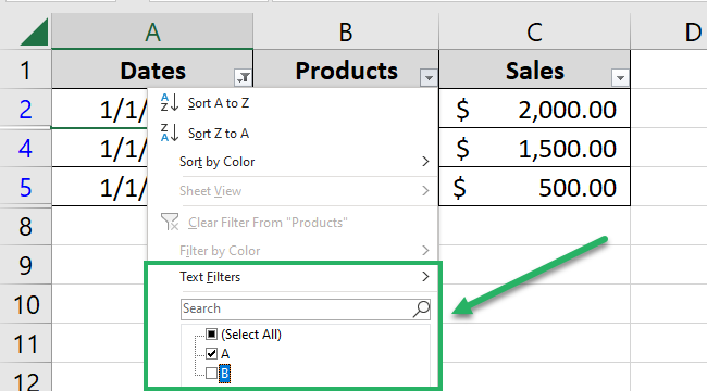
- Now write the SUBTOTAL function as follows:
= SUBTOTAL (
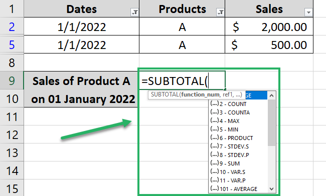
As you start writing the SUBTOTAL function, a list of function_num options appears.
- Select the option for SUM i.e. 9.
= SUBTOTAL (9,
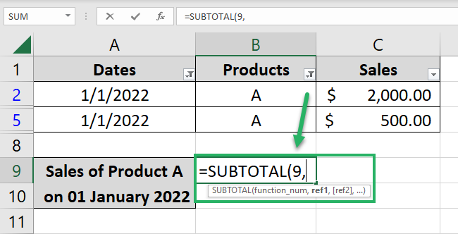
To choose SUM, we have selected 9 and not 109. This is because we want to sum the filtered-out cells + any rows hidden manually.
We don’t have any manually hidden rows here – so the result would be the same under both modes 💁♀️
If you want the SUBTOTAL function to sum up only the filtered-out rows, select 109 as the function_num.
- Select the range to be summed. We are including the entire range i.e. C2 to C7.
= SUBTOTAL (9, C2:C7)
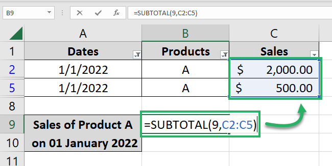
- Press Enter.
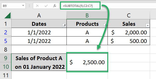
And there you have the sum of $2500 💰
Note that Excel has only added up the filtered values i.e. $2000 and $500. The unfiltered values are not included in the SUM.
Why use SUBTOTAL?
The SUBTOTAL function is a very well-thought and smart function. Here are some reasons why the SUBTOTAL function must be used:
Only includes the filtered data
In the example above, had we used the SUM function, the results would have been as follows:
= SUM (C2:C7)
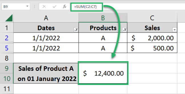
A simple SUM function adds up all the cells – whether filtered or unfiltered 👎
Whereas the SUBTOTAL function only adds up the filtered cells. This way, you can readily change the filtering options to change the results.
For example, change the filter applied on the Dates column from 01/01/2022 to 01/16/2022.
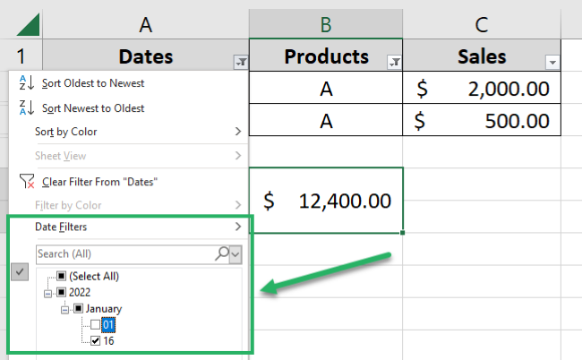
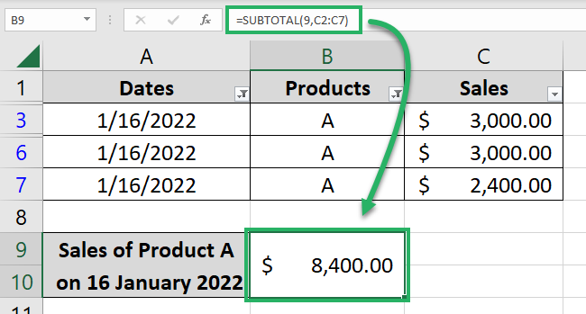
And the sum would also change accordingly as follows:
Excludes any hidden rows
In the example above, we summed up the sales for Product A on 16/01/2022.
Now, what if you quickly want to remove a sale transaction from these filtered cells to see the result then?
- Right-click on that row header (Row 7 in our example).
- Click on Hide from the resulting context menu.
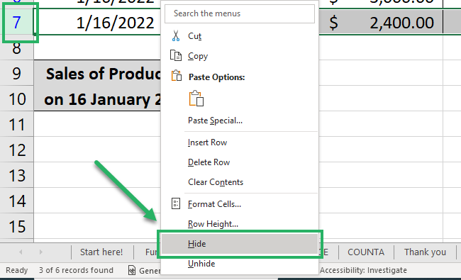
Now the row is hidden, but the results haven’t changed 🤨
That’s because, under function number series 1-11, the SUBTOTAL function adds up the filtered out and the manually hidden rows both.
- Rewrite the SUBTOTAL function as follows:
= SUBTOTAL (109, C2:C7)
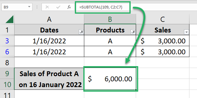
Under function number series 101 to 111, the SUBTOTAL function excludes any manually hidden rows. Our sum now doesn’t include the manually hidden rows (Row 7).
This is not possible with a simple SUM function.
Other uses and examples of SUBTOTAL
You now know when to use simple functions and when to play around with a more versatile – SUBTOTAL function 🎭
With that, let’s look into some more examples of the SUBTOTAL function to better understand how it works in Excel.
SUBTOTAL formula example #1
Let’s see a quick example of using the 101-111 function number series of the SUBTOTAL function.
Here’s the portfolio of an investor who wants to invest in the shares of the following companies.
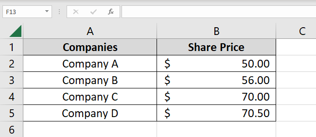
He is certain to invest in Companies A and B. But he will only invest in any one company from Company C and D 🚀
The decision to invest in any company is based on the highest average share price. So which Company should he choose, Company C or D?
Ah, we will find that in a blink.
- Write the SUBTOTAL function as follows:
= SUBTOTAL (
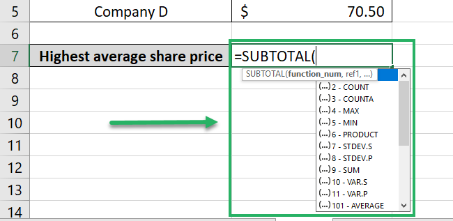
- From the list of function_num arguments, choose 101 (Average)
= SUBTOTAL (101,
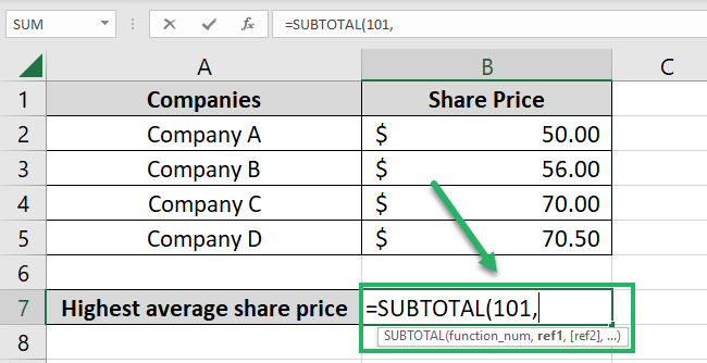
Note that we have chosen the AVERAGE function from the 101 to 111 series 👀
- Select the entire range of share prices from B2 to B5.
= SUBTOTAL (101, B2:B5)
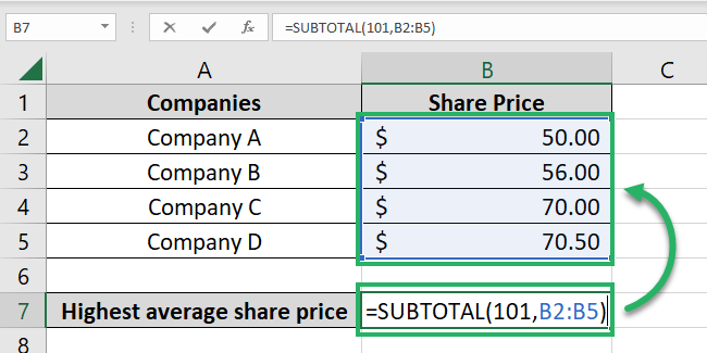
- Press “Enter” and there we have the AVERAGE for all the share prices.
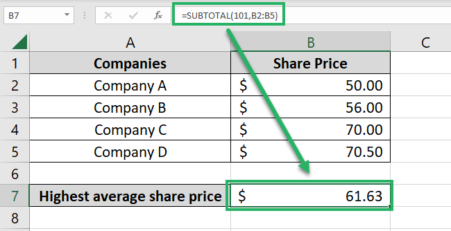
Now, to see which Company’s shares bring the highest average share price:
- Right-click on the row for Company D (Row 5).
- From the context menu that then launches, select Hide.
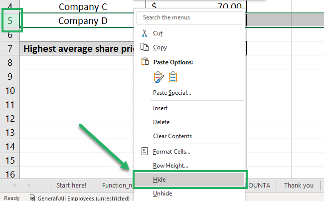
We now have the average share price for the shares of Company A, B, and C only 🤩
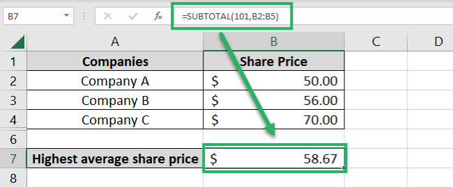
As we have selected the function number series 101 – 111, every time we hide a row, it is excluded from the average share price.
- Now hide the row for Company C (Row 4) in the same way.
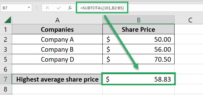
This brings us the average share price for Companies A, B, and D.
And the decision is now clear – investing in Company D gives a higher average share price.
SUBTOTAL formula example #2
Want to see more examples from the SUBTOTAL function? We too.
So, here’s the schedule of a very busy person 👨💼

Starts on the 1st of December and goes up to the 8th of December 2022. How many events are covered these days? Calculate that here.
- Write the SUBTOTAL function as follows:
= SUBTOTAL (
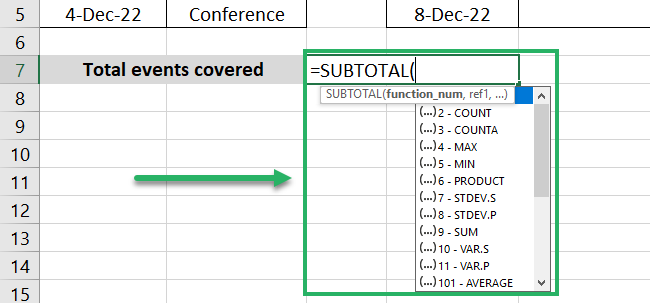
- From the list of function numbers, choose 103 (COUNTA).
= SUBTOTAL (103,
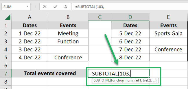
We want to count the number of events only and not the unoccupied days. The COUNTA function counts non-empty cells only 🎯
Note that we have chosen COUNTA from the 101 to 111 series.
- As the Ref1 argument, select the first range of cells i.e. B2 to B5.
= SUBTOTAL (103, B2:B5
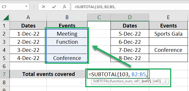
We still have a range left, so let’s include that too.
- As the Ref2 argument, select the second range of cells i.e. E2 to E5.
= SUBTOTAL (103, B2:B5, E2:E5)
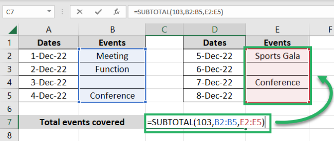
Here we are using the complete syntax of the SUBTOTAL function. Including the optional Ref2 arguments too.
- Press Enter, and there you go.
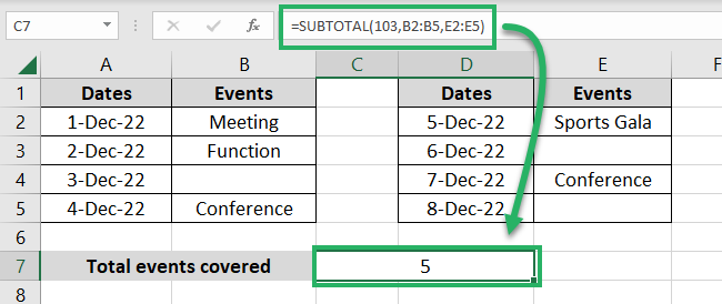
The person has 5 events to attend in a row 🌃
Hold on! What if he chooses to skip the conference of 4th Dec 2022?
- Hide the row for that event (Row 5 in our case).
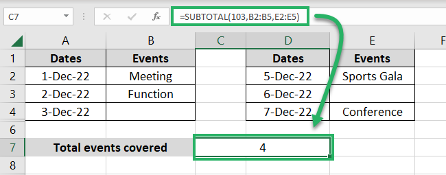
And the count of events now changes to 4.
Had we chosen the function number series 1 – 11, the result wouldn’t have changed to 4 upon manually hiding a row.
That’s it – Now what?
That’s all about the SUBTOTAL function of Excel. We’ve had a super comprehensive discussion on this very versatile function.
Starting from the syntax to its basic application, full syntax application, and multiple other examples. You are a pro at using the SUBTOTAL function now 🥈
If you enjoyed learning about this function, you’d be amazed to know how vast the entire function library of Excel is. Some key functions of Excel include the VLOOKUP, SUMIF, and IF functions.
Want to learn them? Enroll in my 30-minute free email course here to get started. It will teach you everything about these functions.
Other resources
If you enjoyed learning about the SUBTOTAL function, you’d also want to know more about the functions it offers.
Like the STDEV function, COUNT and COUNTA functions, and the MAX and MIN functions of Excel.
