How to Use the SUMIF function in Excel (and SUMIFS)
Without a doubt, one of the most useful functions of Excel is the SUMIF function.
It enables conditional summing up in Excel. And so, you can make sense of large diverse datasets by only summing up the values that meet a specified criterion.
And what if that’s not a criterion but multiple criteria? No worries – to deal with multiple conditions, we have the SUMIFS function to the rescue.
The guide below will take you through everything that you need to know about the SUMIF and SUMIFS functions of Excel👇
So continue reading and download our free sample workbook here to tag along with the guide.
Table of Contents
How to use SUMIF
The SUMIF function sums up only those values (from a defined range) that meet a specified condition. Let’s see how.
The dataset below shows the sale of four products.

Out of this data, can we quickly sum up the sales for “Apple” only? To do so:
- Begin writing the SUMIF function as shown below.
=SUMIF (
- Create a reference to the range (based on which the sum is to be performed).
=SUMIF (A2:A5,
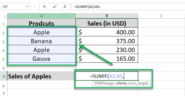
We have created a reference to the cell range A2:A5.
This range contains the product names (and we want to sum up the sales for apples only). So our range is the “Products” column.
- Next, define the criteria based on which Excel must sum the values.
We want to sum up the sales for “Apple” only and that makes our criteria.
=SUMIF (A2:A5, “Apple”,
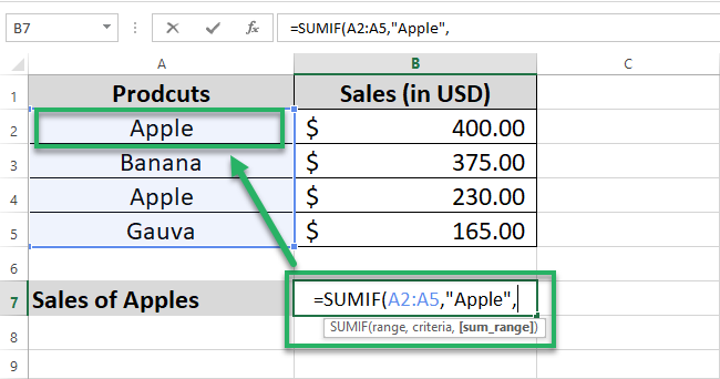
We have defined “Apple” as the next argument. This tells Excel to look out for the word “Apple” in the range specified above.
Don’t forget to enclose the criterion in double quotation marks. Unless enclosed in quotation marks, Excel won’t recognize it as the criterion.
- Create a reference to the range to be summed up (Sales in this case).
As we want Excel to sum up the sales for “Apple”, we are creating a reference to cells B2:B5.
=SUMIF (A2:A5, “Apple”, B2:B5)
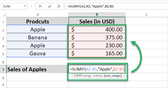
The sum_range is an optional argument.
If left omitted, the SUMIF function, by default, sums up the range instead.
- Hit “Enter” and there you go.
Excel displays the sum of sales of “Apple” only.
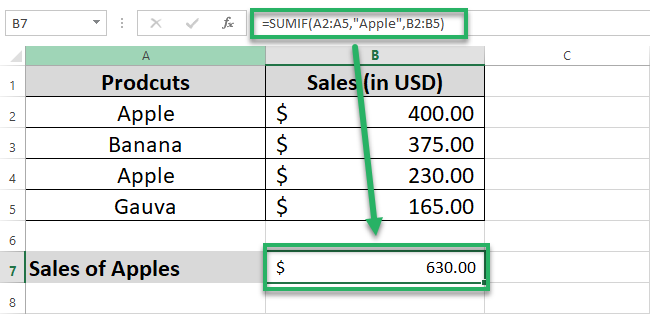
The SUMIF function is only that easy to use. Yes, we love it too 🤍
SUMIF formula examples
The basic application of the SUMIF function is more like child’s play.
But that’s not it – the criteria of the SUMIF function can take different formats. Like the number, text, and date format.
Look into the examples for each criteria format below.
SUMIF with number criteria
Here comes the sales data for three different cities for different months.
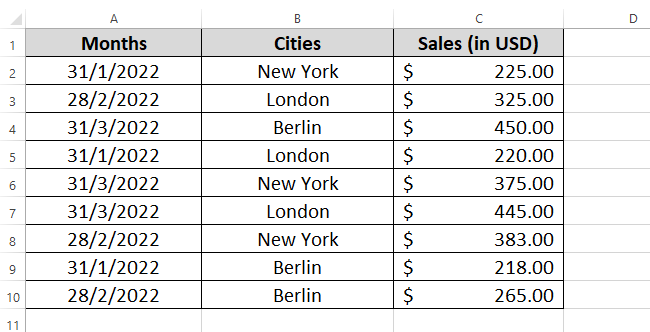
Out of this data, can we only sum up the sales that exceed $225? To do so:
- Start writing the SUMIF function as follows.
=SUMIF (
- Define the range (based on which the cells are to be summed up) as the first argument.
=SUMIF (C2:C10,
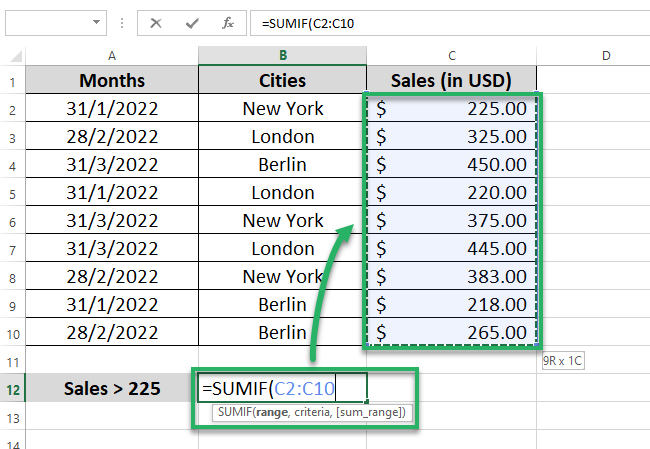
We want to sum up the sales that exceed $225, so our range is sales.
- Define the criteria for summing up the values as shown in the following formula.
=SUMIF(C2:C10,”>225”
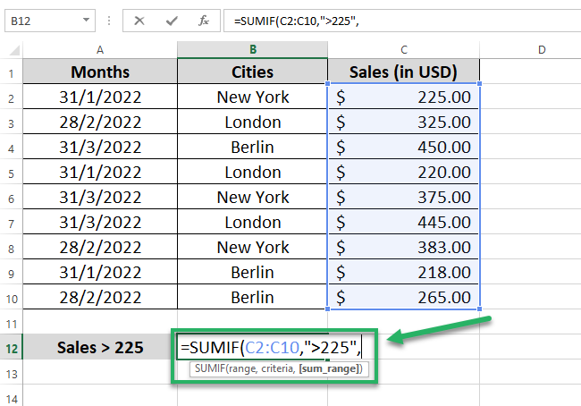
As we want to filter out sales greater than $225, we have defined the criteria using a “greater than” operator (>225).
The SUMIF function supports logical operators (>,<,<>,=) and wildcards (*,?) for partial matching.
- Create a reference to the range to be summed up (the sales) as the third argument.
The sum range argument, in this case, is the same as our criteria range (C2:C10).
=SUMIF(C2:C10,”>225”,C2:C10)
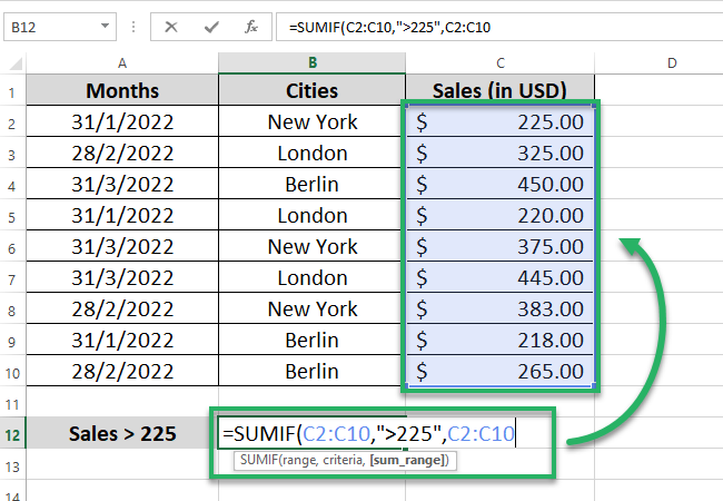
Now, hit enter.
And here comes the sum of the sales that exceed $225.
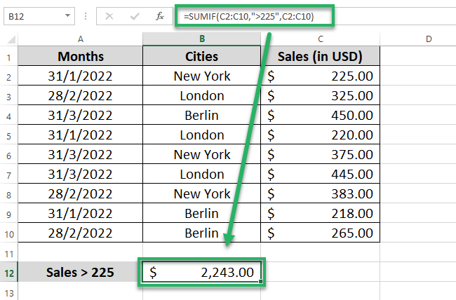
Turns out $2,243 is the sum of all the sales that exceed $225.
SUMIF with text criteria
Continuing with the previous example, what if we want to sum sales of New York only?

- Write the SUMIF function as follows.
= SUMIF (
- Define the range against which the criterion must be evaluated (Cities).
=SUMIF (B2:B10,
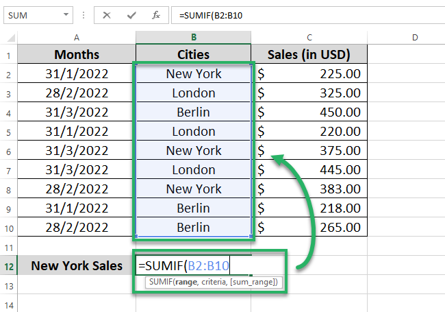
We want to sum the sales for NewYork (a particular city) only so our range is the Cities column.
- Define the criterion for summing up sales.
This time our criteria is a text i.e. “New York”.
=SUMIF(B2:B10,”New York”,
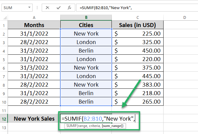
Be very careful about the spelling of the criterion (New York).
If the spelling of the criterion doesn’t match with those in the range, the SUMIF function will fail to sum up the relevant values.
- Select the sum range (the sales) as the third argument.
=SUMIF(B2:B10,”New York”,C2:C10)
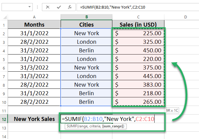
- Hit “Enter”.
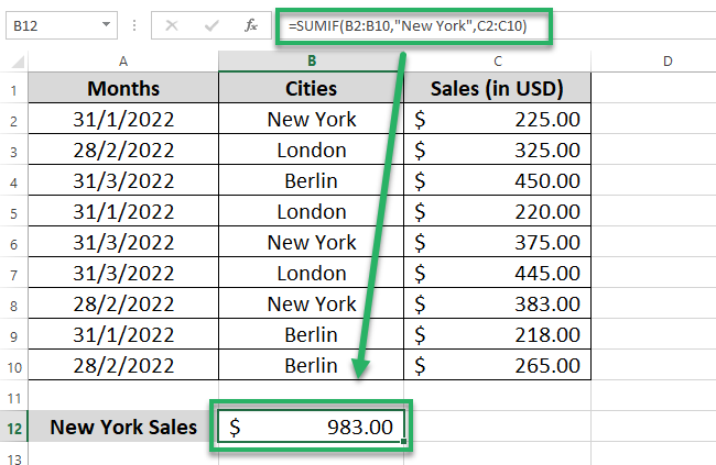
And there you have the total sales of New York City for all the months ✨
SUMIF with date criteria.
So far we’ve learned how the SUMIF function works with a number and text criteria.
It’s time we check if the SUMIF function works with the date criteria too.
With the same data as above, let’s now sum the sales for 31/1/2022 only.

- Start writing the SUMIF function as follows.
=SUMIF(
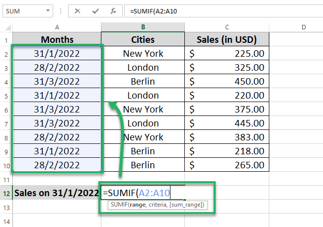
- Define the range as the first argument (Months in this case).
=SUMIF(A2:A10,
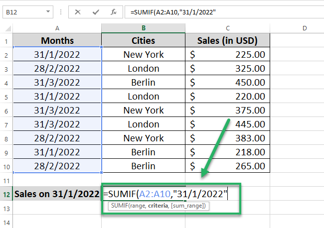
- Define the criteria as “31/1/2022”; the date for which we want to sum up the sales.
=SUMIF(A2:A10,”31/1/2022”,
- Define the sum range (Sales).
=SUMIF(A2:A10,”31/1/2022”, C2:C10)
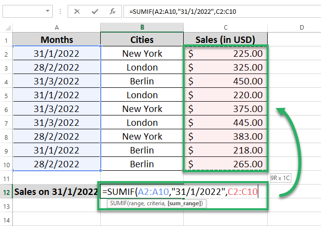
- Press “Enter” to get the results as follows.
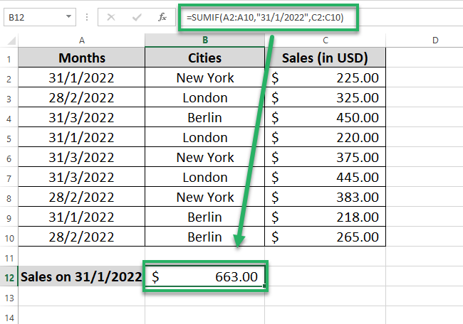
And there you go! Excel sums up the sales for 31/1/2022 only.
Easy peasy, no? 😍
How to use SUMIFS: SUMIF with multiple criteria
Summing up cells in Excel based on a single condition (criterion) was simple enough. But can we achieve the same results with multiple conditions (criteria)?
For that purpose, the SUMIF function won’t come in handy. Instead, you’d have to move to a more advanced version of the Excel SUMIF function – the SUMIFS function.
Let’s go through a quick example to see how the SUMIFS function works in Excel⌛
The SUMIFS function is only available for EXCEL 2007 and onwards.
Using the same data as above, can we sum the sales for New York City that occurred before 31/3/2022? So we need sales that meet the following two criteria:
- Before 31/3/2022; and
- New York
Here’s how we can do it.
- Begin writing the SUMIFS function as follows.
= SUMIFS(
- Define the cell range to be summed up as the first argument (Sales in this case).
=SUMIFS(C2:C10,
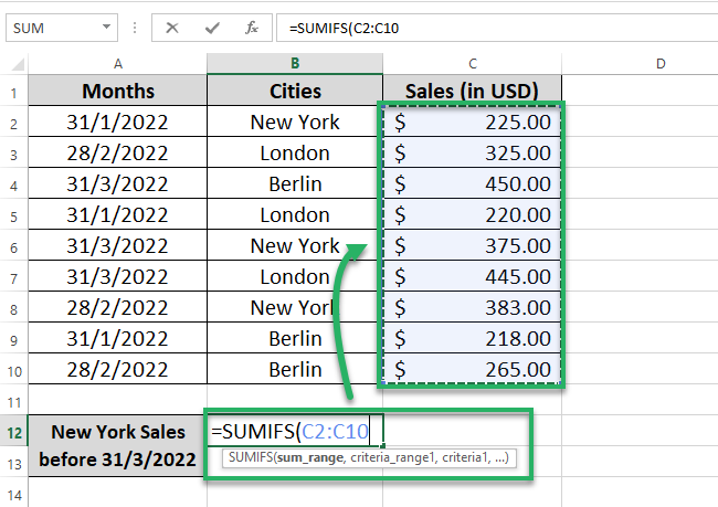
- Define the range for your first criteria as criteria range 1.
=SUMIFS(C2:C10,A2:A10,
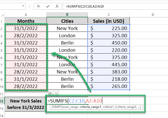
As our first criterion is the occurrence of sales before 31/03/2022, we have created a reference to the column “Months”.
- Define the first criteria (before 31/3/2022) using operators as follows.
=SUMIFS(C2:C10,A2:A10,”<31/3/2022”,
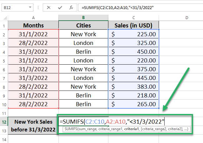
You can use operators with the date criteria too. For example, to define the criterion of (before 31/03/2022), we used the less than operator (<) before the date 31/03/2022.
After we have defined the first criterion, it’s time we move on to the second criterion (New York).
- Select the range relevant to the second criterion (Cities) as the criteria range 2.
=SUMIFS(C2:C10,A2:A10,”<31/3/2022”,B2:B10,
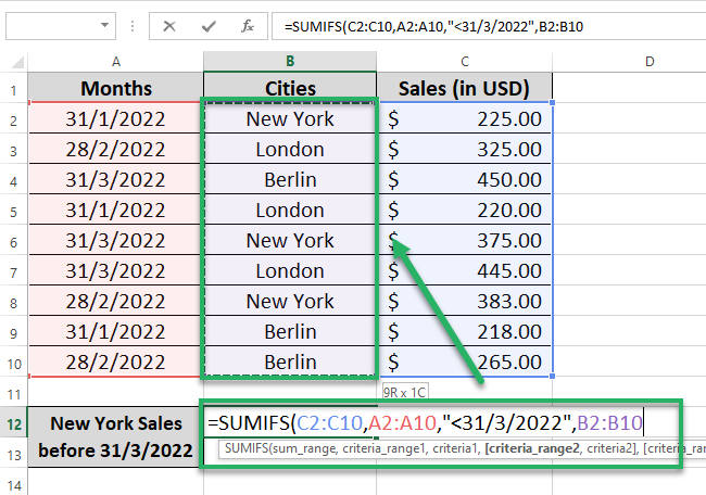
- Define the second criterion (New York) as criteria 2.
=SUMIFS(C2:C10,A2:A10,”<31/3/2022”,B2:B10,”New York”
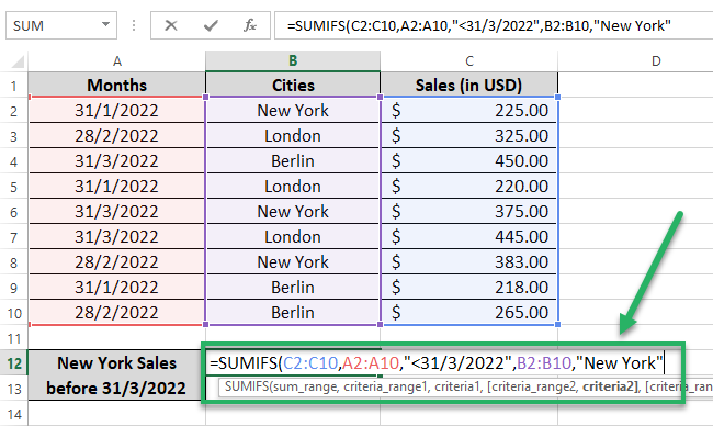
Huh! We are done writing the formula and we are only a hit away from the results now.
- So hit ‘Enter’ to calculate the sum of sales for New York that occurred before 31/3/2022.
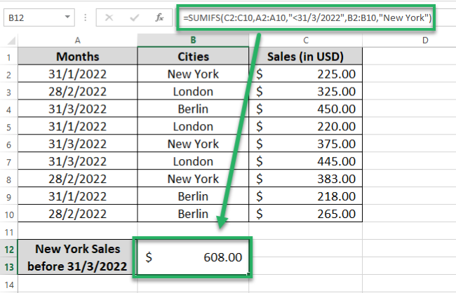
And there you are. The sum of sales for New York that occurred before 31/3/2022 turns out to be $608.
Excel never fails to prove a lifesaver for us, does it?
SUMIF vs SUMIFS: When to use one or another
Both the SUMIF and SUMIFS functions have one thing in common – the ability to sum up numbers conditionally.
But what differentiates both these functions is the room that they have for conditions.
- The SUMIF function is relevant when you want Excel to sum up values based on a single condition only.
For example, when you want to sum the costs that exceed $100. 1️⃣
- However, if you want your dataset to be checked against multiple conditions before the sum is performed, use the SUMIFS function.
For example, when you want to sum the costs that exceed $100 and are fixed in nature 2️⃣
That’s it – Now what?
That’s all about calculating conditional sums in Excel🥂
The guide above explains how to conditionally sum up values in Excel using the SUMIF and SUMIFS functions. It further explains how you can supply different types of criteria (in number, date, and text format) to these functions.
The SUMIF function of Excel is surely a lifesaver. But so are the other core functions of Excel including the VLOOKUP and IF functions.
To learn these functions, enroll in my 30-minute free email course that takes you through these advanced functions of Excel.
Other relevant resources
The SUMIF and SUMIFS function become all the more valuable when used together with operators.
Are you facing problems with greater than / less than operators in Excel? Learn all about them here.
