How to Leave Excel Cells Blank if They Return Zero

Did you ever think about what would be this world like if there were no zeros in it?

Don’t know – hard to imagine. But you can definitely imagine an Excel sheet with no zeroes in it.

If you work with Microsoft Excel, you’d know it’s very common to see undesired zeros around your sheet. Sometimes, this might be the result of a formula or of importing data into your sheet from external sources.

In either of the cases, you can help this situation with a variety of methods – all of which are explained in the tutorial below 👇

So, grab your free practice workbook for this guide now and tag along with me till the end.

Table of Contents

Worksheet Settings: Don’t display Zero Values

Although there are many methods to remove zeros from Excel datasets by leaving cells blank, this one is the easiest and has a blanket effect.

Let me show you how.

Here’s a dataset in Excel that’s cluttered with zeros.

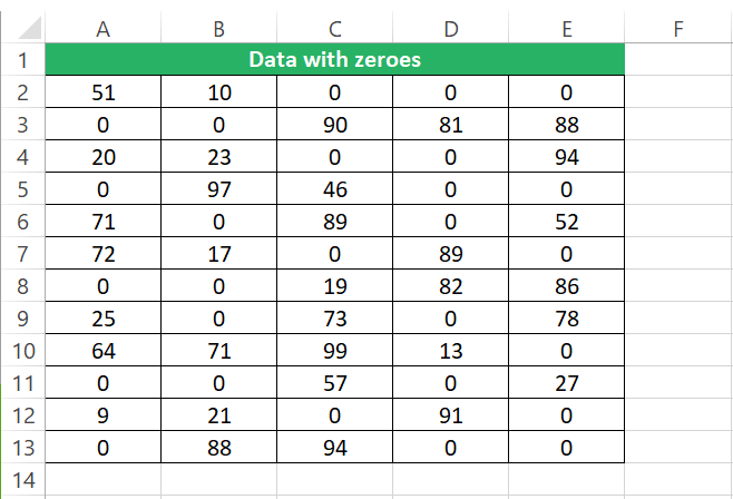
To make sure these zeros are not displayed on the face of your sheet:

Step 1) Go to the File tab.

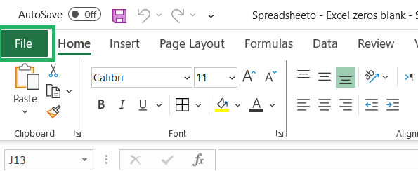
Step 2) Go to Excel Options.

Step 3) Go to the Advanced settings from the pane on the left.

Step 4) Scroll down to “Display options for this worksheet”.

Step 5) Uncheck the option “Show a zero in cells that have zero value”

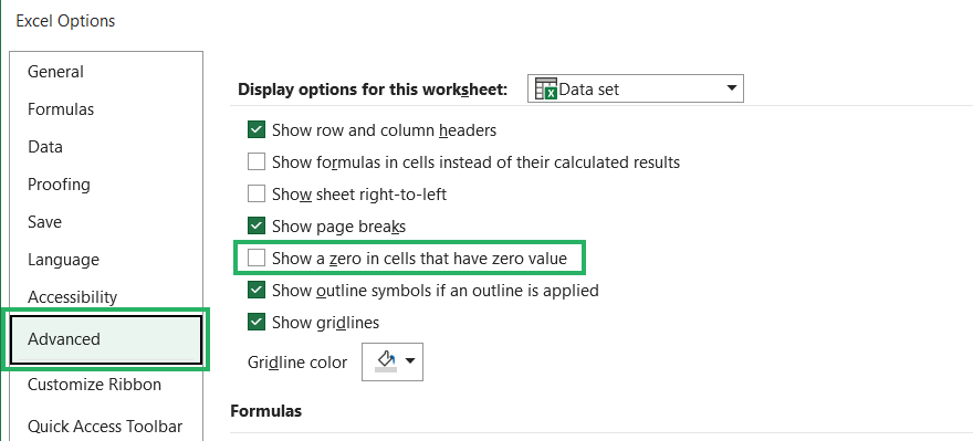
Step 6) Press okay,

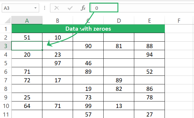
Coming back to your worksheet, you will see the zeros have vanished.

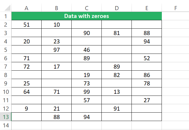
Easy and quick, right?

However, the zeros have only vanished from the face of the sheet, but they are still there 👀

Pro Tip!

Despite how easy and quick to use this method is, it has the following two drawbacks:

• These settings only apply to the active worksheet and not to a whole workbook. You must reapply them for each worksheet.
• These settings apply to the entire worksheet and not to a specific cell range from a given worksheet. So, it’s only useful if you want it applied to the whole sheet.

White them out using Conditional Formatting

You can also get rid of the zeros appearing on the face of your worksheet by using conditional formatting.

Let’s do it now to learn now.

Step 1) Select the cells from where you want the zeros removed.

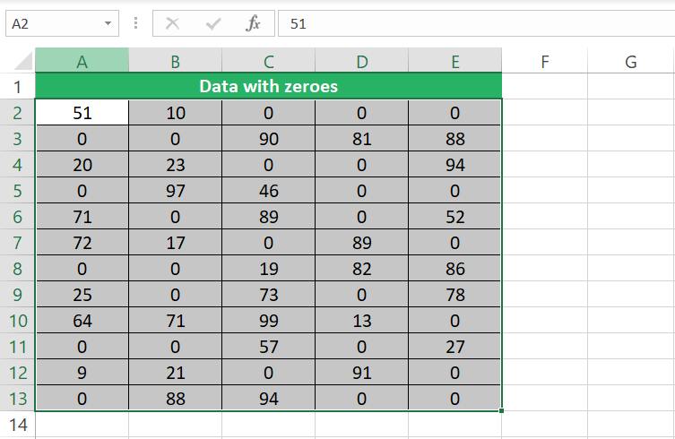
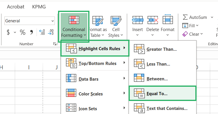
Step 2) Go to the Home tab > Styles group > Conditional Formatting.

Step 3) From the Drop-down menu that appears, select Highlight Cells Rules > Equal to.

This will launch the Equal to dialog box as shown below 🧾

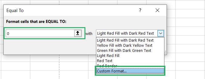
Step 4) Within the ‘Equal to’ rule dialog box, set the equal to value to 0.

Step 5) From the Format options, launch the menu and select Custom.

Clicking on custom format will take you to the Format Cells dialog box.

Step 6) From the Format Cells options, go to the Font tab.

Step 7) Select Color > White color 🎨

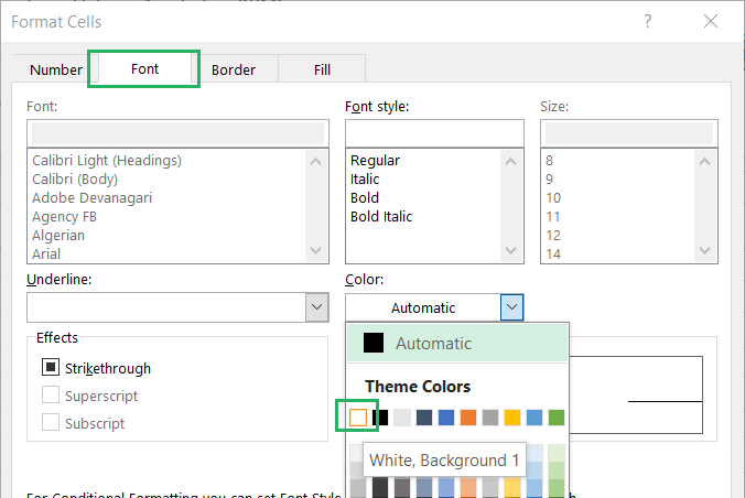
Step 8) Press okay to see the magic on your sheet.

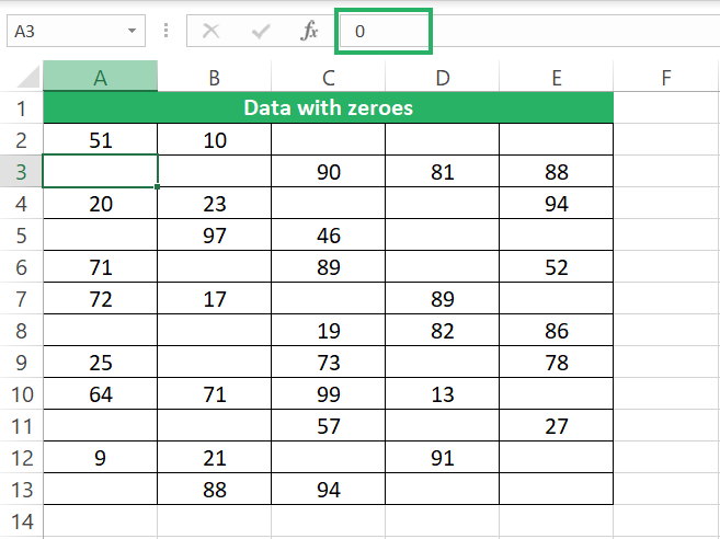
The conditional formatting rule has filled in all the cells that contain zero with white color. Since the background color of the sheet is also white (no color), it seems like the cell is blank.

Technically, the zero is still there, it has just been whited out.

Custom Format

Like we apply different formats to numbers including Accounting, Currency, and other formats, you can also devise a format of your own that makes the zeros disappear 🔢

Wanna see how? Check this out.

Step 1) Select the cells where you want to apply the custom format to remove the zeros.

Step 2) Go to the Home tab > Number group > Number formats.

This will launch the Number Format dialog box as below.

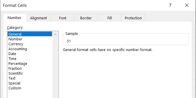
Step 3) From the pane on the left, select Custom Format.

Step 4) In the type box, type the number format as

Pro Tip!

This custom format takes four types of data formats, each of which is separated by a semi-colon.

• Positive number format (denoted by the first zero). Excel will present positive numbers as they are.
• Negative number format (denoted by the second zero with a minus sign after a semi-colon). Excel will present negative numbers with a preceding minus sign.
• Zeros (that we have omitted altogether).
• Text format (denoted by @ sign after the third semi-colon)

You can change the format for any of these data types here. For example, if you altogether omit the negative number format, all negative numbers will vanish from the face of your sheet.

Similarly, you can give the positive number format as +0 to have a + sign appearing before all positive numbers in your sheet.

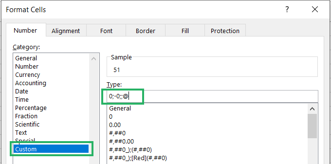
Step 5) Click the okay button to have the formatting applied.

Again – this is only a format change. The zeros are still there.

IF function

One way to get rid of the zeros in your data can also be to use the IF function. However, this method can only be used with the zeros resulting from formulas 🚀

For example, I have some formulas running behind numbers here in Excel.

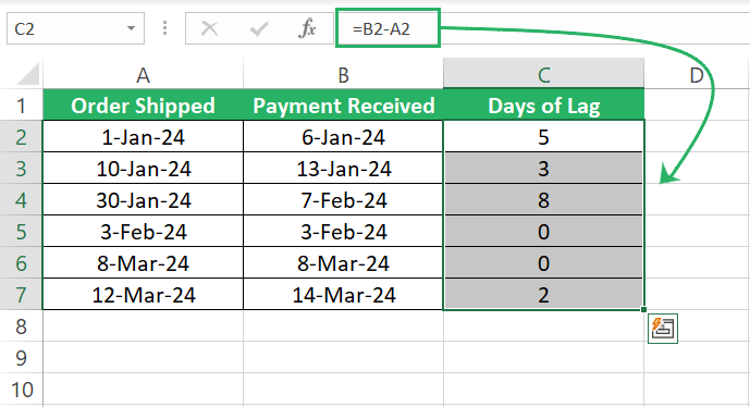
The above image shows the data for when an order was shipped to my customers v/s. when was the payment received from them.

To find the number of days in between, I have deducted the former date from the latter date in Column C.

For those orders that were shipped and the payment was received on the same day, Column C shows zero. However, I don’t want zeros in my sheet – instead, I want the text “No Delays” in its place.

Easy – we will wrap these formulas in the IF function and specify the desired text (“No Delays”) as value_if_true.

Step 1) Write the IF function as below.

= IF (B2-A2=0, “No Delays”, B2-A2)

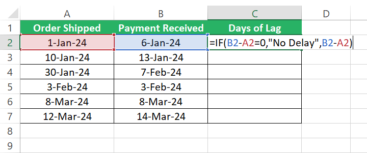
This tells Excel to check if the difference between both dates (B2-A2) equals zero. If it does, return “No Delay” (could’ve been any text of your choice, or even blank). And if it doesn’t equal zero, then return the result of B2-A2.

Step 2) Press Enter to see the results.

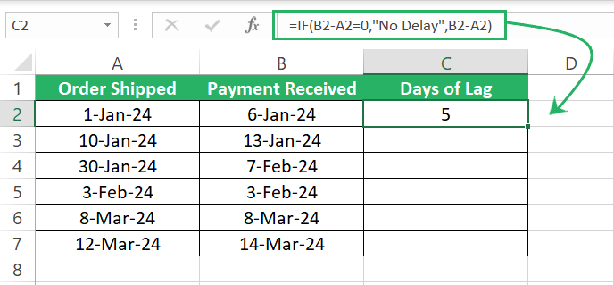
Step 3) Drag the same down to the entire column.

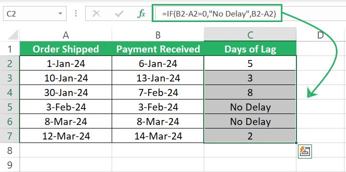
There you go. All zeroes are replaced with whatever you want to see in your sheet.

Show dashes in place of zeros

This method doesn’t hide zeroes, nor does it remove them.

It only replaces them with a dash. It is commonly used for accounting numbers where these dashes represent the meaning of Nil 💻

Here’s how to do it.

Step 1) Select the data set.

Step 2) Go to Home tab > Number > Comma Style.

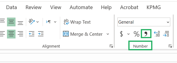
This applies the comma-style formatting to the selected cells. And guess what?

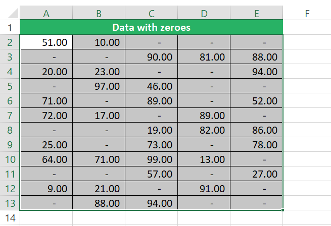
All zeros from the dataset have been replaced with dashes.

It is important to note that the zeros from the dataset have not been removed. They are still there, only the way they are presented has been changed.

And if anytime, you want the zeros in your data back, you can simply change the formatting to General from Home tab > Number Group > Number formats. The dashes will again be replaced by zeros 🎯

Replace Zeros with blanks

All the above methods explain how you can hide zeros from appearing on the face of your sheet. However, none of these methods discuss how can you remove zeroes from an Excel sheet in a hassle-free manner.

Don’t worry – this section will 🧐

So here we have some numbers in an Excel sheet (many of which are zeros that we no longer want there).

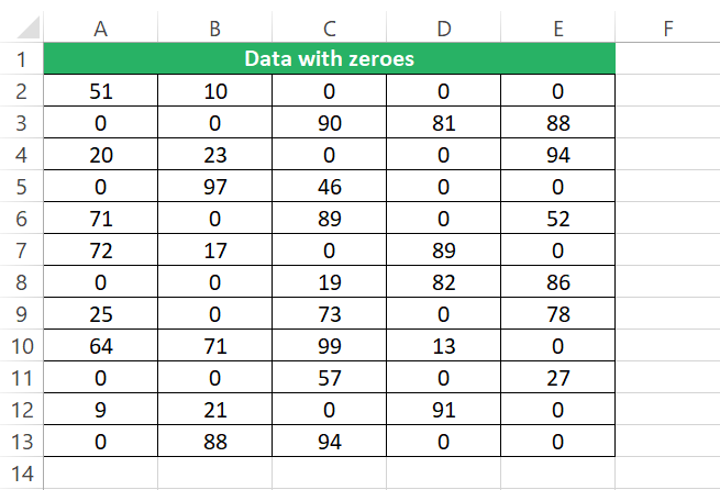
Now, to remove these zeros in their entirety, we will use the Find & Replace tool of Excel.

Step 1) Press the Control key + H to launch the Find & Replace tool.

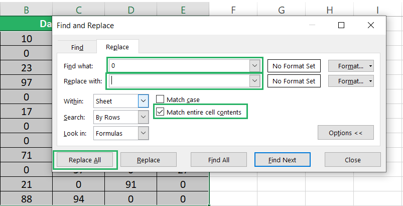
Step 2) Go to the Replace tab within it.

Step 3) Next to the “Find What” box, write 0.

Step 4) Leave the “Replace With” box empty since we want the zeros to be replaced with blanks (nothing).

Step 5) Check the option to “Match entire cell contents”.

Step 6) Click on the button “Replace All”.

Here are what the results look like 🤩

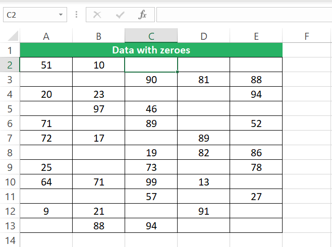
All the zeros from this sheet have been replaced by blanks.

Pay attention to the formula bar to see that the cell is empty – this method removes the zeros instead of merely hiding them.

Conclusion

While zeros can be problematic most of the time. There might also be times when you need them in your sheet to sort things out.

Working out zeros in Excel the way you want them is an art, if not a science, and some of my dedicated Excel tutorials (as listed below) will help you master it in no time. Must give them a read.

• How to Add Leading Zeros in Excel: Best Methods (2024)
• How to Fix the #DIV/0 Error in Excel (Step-by-Step)