How to Calculate a Range in Excel
(Real Examples)

Understanding how ranges work in a spreadsheet is crucial to strengthening your grip on Excel. You can perform large calculations across a set of cells in one go using ranges 🧾

You need to access ranges in different scenarios, whether you’re selecting data for a formula, chart or SPILL function 📊

In this tutorial, we will learn basic and advanced techniques used to calculate ranges in MS Excel. Get our free sample workbook below to practice ranges now.

Table of Contents

What is a range?

In simple words, range refers to the difference between the highest and lowest values in a dataset.

This means, that if you had a dataset computing the total sales made in a month, where the highest sale was 9000 and the lowest was 500, the range of this dataset would be the difference between the two ➖

Range: 9000-500

The same concept is implemented in Excel where you find the range of a dataset by subtracting the highest values from the lowest values 🔽

Your range can take the shape of any form. this means you can create vertical, horizontal, mixed range or even a multiple selection range where the range consists of random cells in the sheet.

How do you calculate range in Excel?

The process of calculating range is straightforward, even if you are dealing with hundreds of rows. There are a couple of formulas in Excel that work perfectly in finding out ranges 🧐

These include the MAX, MIN, SMALL, LARGE, RANK, COUNTA, COUNTIF, MEDIAN and IF. We will see examples of the most commonly used functions to find the range 🔍

Find maximum and minimum values

Say, you have the following sample dataset of a company with its sales records of the previous year including duplicates. The representative needs to figure out the sales range to draw useful insights for the next year’s sales 💲💲

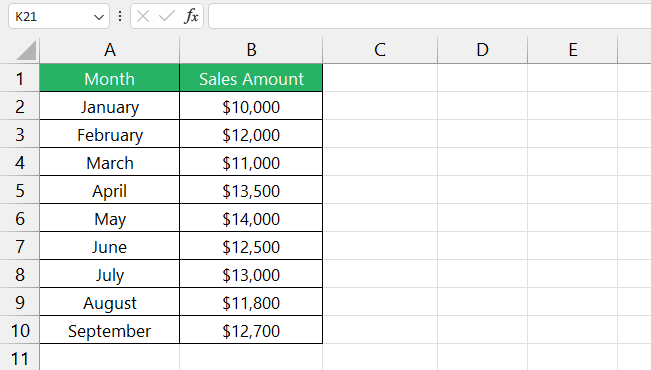
To do that,

Step 1) Select cell C2.

Step 2) Type in the following range formula

Step 3) Press Enter.

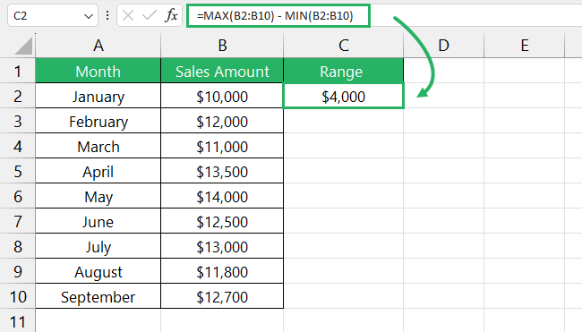
The minimum function and maximum function return the range of the dataset.

The logic here works such that the MAX function returns the maximum values of the data set while the MIN function returns the minimum value of the data set. We then find the difference of the two values which gives us our range of the dataset.

That wasn’t difficult now, was it? 😀

Find small and large values

You can find a range by extracting its maximum and minimum values but what if you want to see n number or nth number of smallest or largest values in the dataset? 🤔

For that, we use the SMALL and LARGE Excel functions. Their syntaxes are given below.

where,

array refers to the range of cells you want to find values in

k refers to the position of the smallest number in the given array, i.e., if you want to find the 4th smallest value, k would be 4.

Similarly,

where,

array refers to the range of cells you want to find values in

k refers to the position of the largest number in the given array.

We are using the same sample data as in the above example 🔼

We will first find the smallest values and then the largest values.

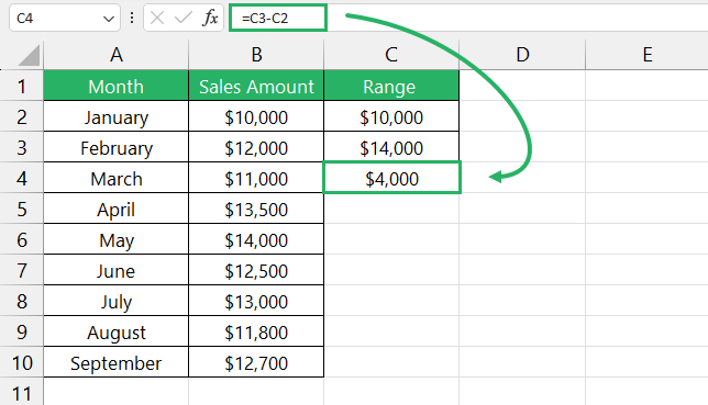
Step 1) Select cell C2.

Step 2) Type in the following formula

Step 3) Press Enter.

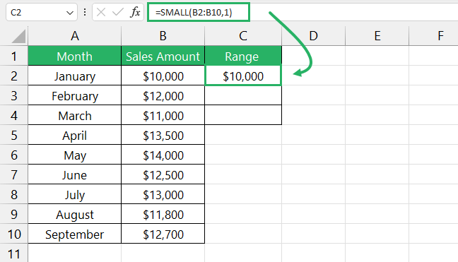
Repeat the same steps for the LARGE function 🔁

Step 1) Select cell C3.

Step 2) Type in the following formula

Step 3) Press Enter.

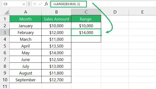
Step 4) In cell C4, find the difference between the two values ➖

Step 5) Press Enter.

And voila! You have your range of the dataset 😃

You can also find multiple small and large values using the same formula. Simply copy it across cells using the Fill Handle and change the value of k to the number you want.

How to calculate conditional range in Excel?

In practicality, finding the range of a company’s dataset wouldn’t be as straightforward as we saw above. You might need to find the range within certain limits or conditions.

That is where conditional ranges become useful. You can combine different functions to create certain conditions for your range 🧾

For example, you might need to find the lowest value in the dataset but that value must not be smaller than 100 – in this case, you would need to apply a condition.

There are multiple ways to get the same result. Let’s first see a simple IF array formula example to get a hold of the concept 😀

We have the following sample data.

Step 1) Select cell C2.

Step 2) Type in the following formula

Step 3) Press Enter.

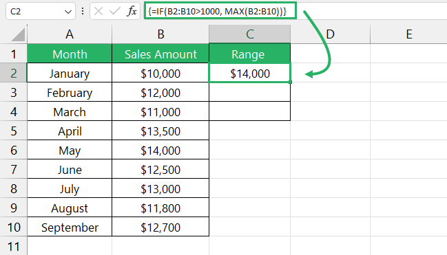
Step 4) Type in the following formula in cell C3 ⌨

Step 5) Press Enter.

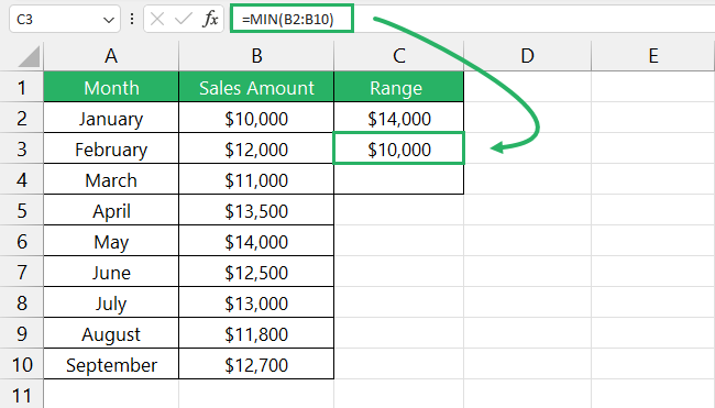
Step 6) In cell C3, subtract the two values.

Step 7) Press Enter.

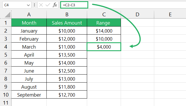
This returns the range of the dataset provided it meets the given condition. You can provide the value you would like to display if the condition is false in the IF function ❌

You can also calculate conditional ranges using the MAXIFS or MINIFS functions. Since syntaxes of both the functions are same, let’s see MAXIFS syntax below:

where,

max_range refers to a range of cells from where we want to find the maximum value

criteria_range1 refers to the range you want to evaluate

criteria1 refers to the condition to be used on the range – it can be a numeric value, text string, or even an expression

Let’s now see a quick example of MAXIFS and MINIFS in action 🧐

We have the following sample data.

Step 1) Select cell C2.

Step 2) Type in the following formula.

Step 3) Press Enter.

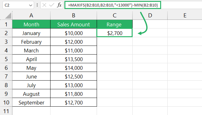
The formula works such that it checks for maximum value in the range that is less than 13000, i.e., 12700. We then find the difference between the highest and lowest value in our worksheet, i.e., 10000 from 12700 which returns 2700.

You can tweak the formula as you like to ensure the range passes a specific condition check. Pretty easy, right? Try it now! 😃

Conclusion

In this tutorial, we saw what a range is in Excel and how you can calculate it using different methods. Having a strong understanding of range manipulation is a critical skill in data analysis.

The concept is easy to grasp, all you need is practice, especially with conditional ranges. If you want to know more about ranges and their formulas, give the below articles a read 📑

How to Name a Range in Microsoft Excel: Step-by-Step (+ Name Manager)

How to use the MIN and MAX Functions in Excel: 2024 Guide

How to Use MAXIFS and MINIFS in Excel: Step-by-Step (2024)

We hope you enjoyed reading this article as much as we enjoyed creating it 🤗