How to Name a Range in Excel: Step-by-Step (+ Name Manager)

Excel is all about storing data and doing something with it. And to make data storage and manipulation easier, Excel allows users to name their data.

You can name different ranges (or arrays) in Excel and the Excel Name Manager will store them for you. Once saved, you can refer to that range of cells simply by using its name.

So instead of referencing a range like this =SUM($A$2:$C$250), write the name you gave it, which could be something like this =SUM(Prices).

Looks much easier, right? 💡

Practicing something in real-time can make you 10x faster at it. And you can master naming ranges in Excel with our sample workbook for free. Grab it here.

How to name a range in excel

A named range can save you a lot of time and confusion. And if you haven’t used it before, take my word for it – it’s very easy to create a named range.

It literally takes less than five seconds – unless, of course, the name you assign is extremely long 😅

Let’s see a simple example of naming a range below.

We have the following data.

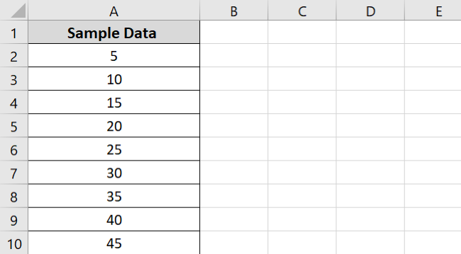
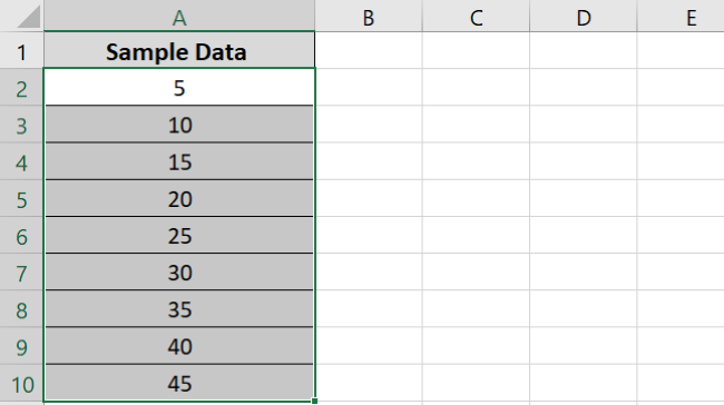
I want to name the range A2:A10 as ‘Tableof5’.

For that:

1. Select the range.

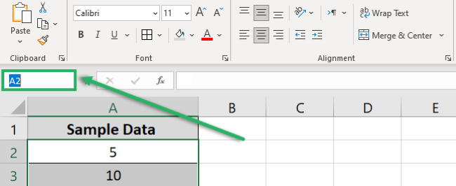
2. Click in the Name Box

3. Assign a name to the cell range.
4. Press Ok.

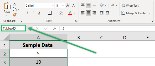
The selected range has now been named.

Excel will show you the name of the range when you select it.

Important note:

Note that the name of a range cannot contain space. If you add space in the Name Box, Excel will show an error prompt:

Similarly, the first character of the name cannot be a digit. And names cannot have any other symbol other than period, backslash, and underscore character. Also, the name must not exceed 255 characters.

How to use a named range in a formula

Named ranges make writing formulas easier and quicker. Usually, you would type a formula, select all the cell references and then press Enter.

But with named ranges, you just need to enter the name of the range in place of the arguments. And it’s done 🤓

Let’s see how to use a named range in the formula below.

We will use our previous data set for this example.

We want to calculate the AVERAGE of the values of the sample data. For that:

1. Name the range you want to use in the formula.
2. In a cell, type in the formula.

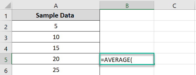
3. Enter the named range in place of the argument.

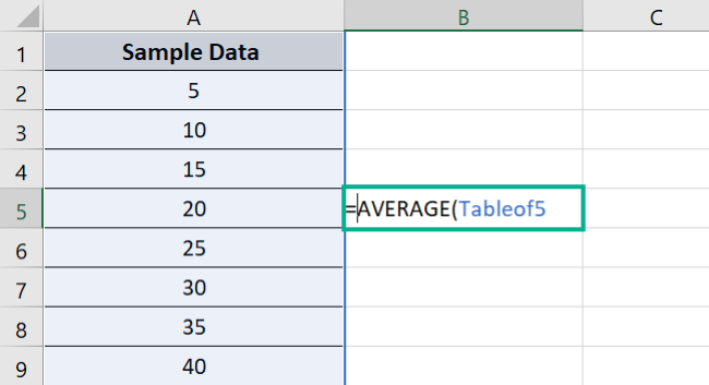
As evident, the formula immediately picks up the named range.

4. Press Enter.

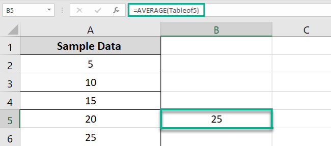
Excel returns the AVERAGE of the named range.

Pretty easy, no? 😃

How to use the name manager in excel

Using names for ranges can be really useful – especially when working with an exceptionally large worksheet.

But it can be equally confusing too.

You can’t possibly readily remember the names of 32 ranges and their exact location. And figuring it out manually will leave you with no time.

Luckily, we have the Name Manager in Excel for this purpose.

As evident from the name, the Excel Name Manager is like the index page where all named ranges and cells are stored. You can also find the location of all named ranges in your Excel worksheet.

Let’s understand the Name Manager’s work in more detail below.

To open it:

1. Go to the Formulas Tab.
2. Select Name Manager from the Defined Names group.

3. The Name Manager dialog box appears.

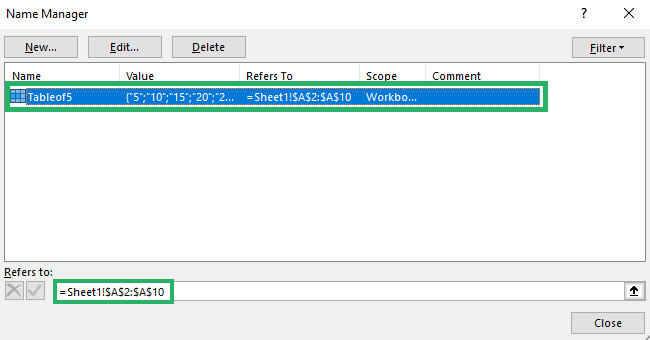
The Name Manager shows our previously created named range. It also shows which cells the named range refers to.

PRO TIP! 

You can open the Excel Name Manager in seconds using the shortcut ALT + M + N. Cool, no? 😎

You can find all your named ranges in one place, thanks to the Name Manager. This makes it extremely useful, especially if you have plenty of named ranges.

There’s also a Filter button at the top right corner of the dialog box. It offers a menu of options that you can choose to perform different operations.

Edit named ranges

Just like adding and deleting named ranges, you can edit them too. You can access the Edit feature from the Name Manager dialog box.

You can edit the name of the range, change its reference, and even add comments.

Say, we want to change our named range ‘Tableof5’ to ‘Multiplesof5’.

For that:

1. Click Edit from the Name Manager dialog box.
2. The Edit Name dialog box appears.

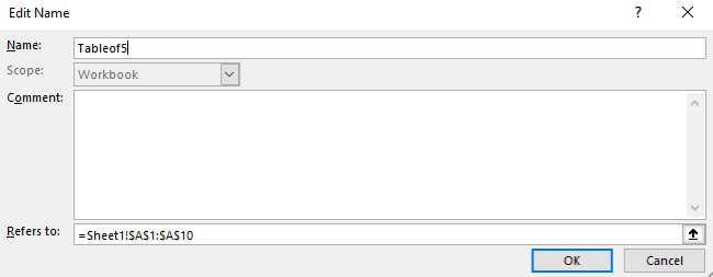
3. Click in the Name box and enter the desired name.
4. Press Ok.

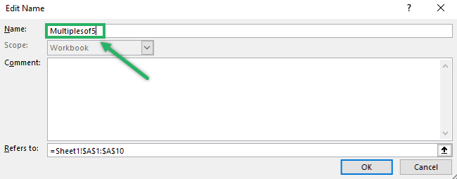
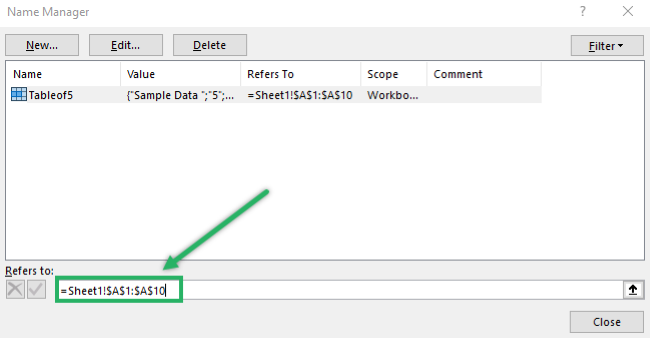
You can also change the references if you want to add or delete a field from the ‘Refers to’ box. It is at the bottom of the Edit Name dialog box.

Or you could do it directly from the Name Manager dialog box to save a click or two.

And that’s all about Editing named ranges in Excel 🤓

How to delete named ranges in Excel

Deleting named ranges is as simple as creating one. To delete it:

1. Open the Name Manager dialog box.
2. Select the named range you want to delete.
3. Press the Delete button at the top.

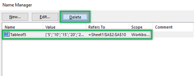
4. Excel will show a warning prompt.
5. Press Ok.

The selected named range will be deleted.

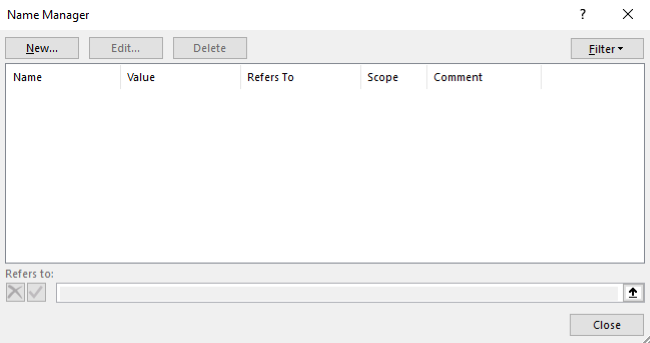
That was easy, right? 😀

That’s it – Now what?

In this article, we learned how to create named ranges in Excel. We also saw what purpose the Name Manager serves and how to edit and delete named ranges.

The named range is a very powerful and resourceful tool of Excel, especially when you have to store tons of data and refer to it several times. It lets you specify a name for each range and this makes working so convenient.

Instead of adding cell references of a range, you can simply use the name of the range in the argument. It is not only faster but easier too.

But to use named ranges in formulas, you need to know the functions first 😅 Worry not, we’ve got a solution to that as well.

Good functions to pair with named ranges are VLOOKUP, IF, and SUMIF. You can learn them for free in my 30-minute Excel course – delivered right to your inbox.

Other resources

In addition to ranges, you can also name data tables in Excel. And although naming a group of cells is easy, people often make errors while using them.

Most importantly, if you misspell the name of the named range while entering it in a function, you’d get a #NAME error. How do you fix that? Check our tutorial!

Frequently asked questions