How to Get a Column Number in Excel: Easy Tutorial
An Excel sheet is two-dimensional – it has rows and columns. By default, row headers in Excel are numbers, and column headers are alphabets.
As the data in your Excel sheet starts to grow in width, the number of columns grows. And this might make it difficult for you to track down a column by its number.
The article below explains different methods of how you can get column numbers in Excel. Also, it focuses on how column numbers might help you in your Excel jobs.
So stay tuned till the end! 😀
Practice the examples shown in the article below by downloading the sample workbook here.
Table of Contents
How to get column number with the COLUMN function
If you have never before heard of the COLUMN function, it’s alright. Most Excel users have not.
The COLUMN function of Excel is designed to return the number of a column in Excel.
To find the column numbers for different columns in Excel, see the example below.
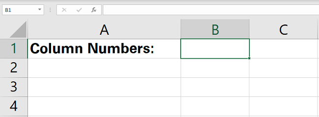
1. Write the COLUMN formula.
=COLUMN()
And this is it!
The COLUMN function has just one argument – the reference argument. Interestingly, this argument is also optional.
If omitted, Excel deems it equal to the Cell reference where the formula is written.
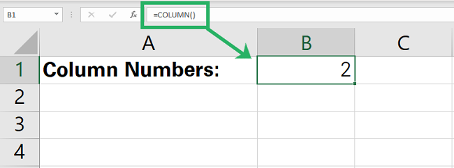
We had omitted the argument, so Excel set it equal to Cell B2. Column B comes second in the sequence, so Excel returned ‘2’ as the Column number.
Let’s see this the other way around.
2. Set the reference argument to AAX10.
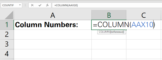
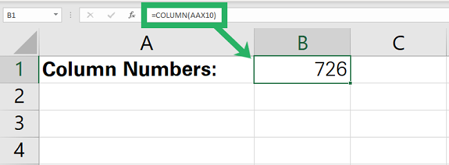
This time Excel returns column number 726. This means Column AAX is the 726th Column of Excel.
How many columns are there in an Excel Sheet?
The last column of an Excel worksheet is Column XFD. So how many columns are there in a single worksheet?
Let’s do it quickly!
- Press Ctrl + the right arrow button ➡️ to fast forward to the last column of Excel.
- Write the Column formula.
=COLUMN()

16384 Excel Columns to each worksheet.
Let’s double-check the same from Google! 😆

Examples of uses for the COLUMN function
Why would anyone want to use the COLUMN function? The examples below tell why.
Example 1:
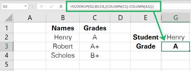
The image below shows the grades of a few students (to the left).
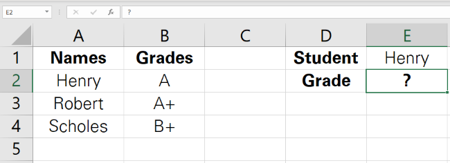
To the right side, we want to fetch out the grades for Henry. Easy solution = VLOOKUP.
1. Write the VLOOKUP function as follows.
= VLOOKUP (E1,

The lookup_value is referred to as Cell E1 because it contains the name of the student to look the result for.
2. Refer to the table array where the lookup and the return values are.
= VLOOKUP (E1, A1:B4,

3. For the col_index num argument, nest in the COLUMN function as follows:
= VLOOKUP (F1, A1:B4, COLUMN(B1))
The col_index num argument refers to the column from where the value is to be returned.
And this has to be the number of the column starting from the first column of the table_array.

We want the Grades of Henry to be returned. Grades are listed in column B, so we have referred to Cell B1 (any cell from Column B).
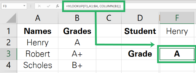
Instead of manually counting the columns, let the COLUMN function do the job.
The VLOOKUP function needs the column number starting from the table array. If the table array starts from any column other than the first column, the above function might not work.
For example, what if the table array above started from Column B and not A?
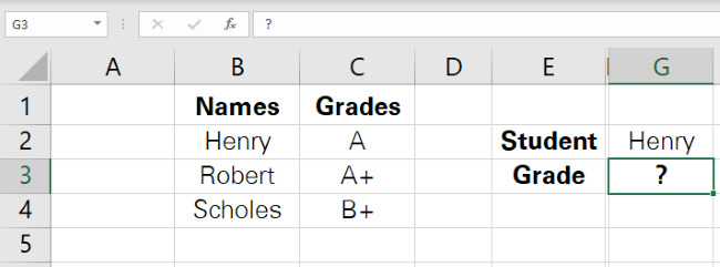
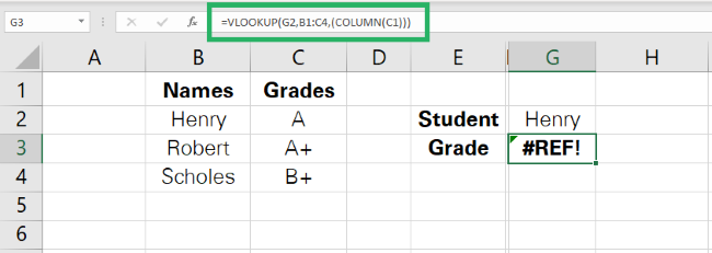
1. Write the VLOOKUP function as above, and it’d fail to function.
=VLOOKUP (G2, B1:C4, (COLUMN (C1))
It will take the col_index num argument as 3 (Column number of Column C).
Whereas, our table range has only two columns.
2. Deal with such a situation by changing the COLUMN function as follows.
= COLUMN(C1) – COLUMN(A1)
Subtract the number of the column before the table array (Column A) from the return value column (Column C).
3. Rewrite the VLOOKUP function as below.
= VLOOKUP (G1, B1:C4, COLUMN(C1) – COLUMN(A1))
Here are the results!
Example 2:
The COLUMN function is not only meant to find the number of a single column. You can also use it to find the number of multiple columns at once.
The data below shows the monthly utility bill of a household.

To find the accumulated utility bill for each month, let’s apply the COLUMN function.
1. Write the COLUMN function as follows.
=COLUMN(A2:F2)

The range A2:F2 tells the number of months for which we need the accumulated bill.

2. Multiply it with the particular cell of the monthly bill.
= H3 * COLUMN(A2:F2)
The cell reference is set to H3 as it contains the monthly bill.

Check out the results.

It only takes a single click for Excel to compute the bills for all the months.
When the reference argument of the column function is defined as a range, the output is an array.
Caution! The SPILL Error:
If the cells of the array are not vacant before the array function operates, Excel gives the #SPILL! Error.

Show column number instead of letter
Only if Excel labeled both the rows and columns with numbers and not alphabets – things would have been much easier!
If you think like that, let’s do it for you.
To change the column letter to numbers in Excel, continue reading.
1. Go to File > Options
2. This opens up the Excel options dialog box.
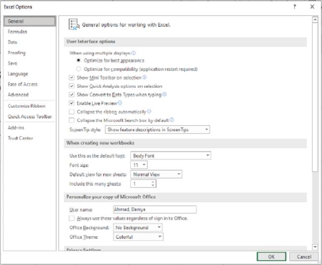
3. Go to Formulas.
4. Under the tab, ‘Working with Formulas’, check the box R1C1 Reference Style.
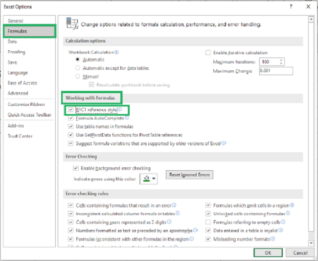
And swish! Magic. The reference style of columns has changed. 😉
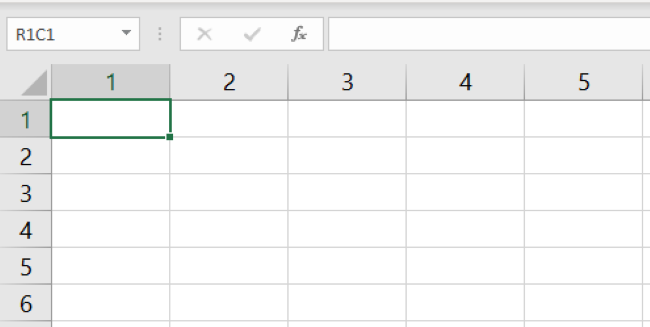
Your Excel worksheet looks all new with a new reference style! Both columns and rows are labeled by numbers.
The R1C1 style reference indicates the Row number and Column number. Accordingly, the cell references will automatically change.
For example, the traditional Cell reference C5 has now become R5C3 (Row number 5 and Column number 3).
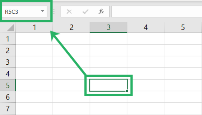
This way, you can easily track down the number of columns.
That’s it – Now what?
By now, we have learned to find the column number in Excel through the COLUMN formula, to nest the COLUMN formula in VLOOKUP, and also to change the Column reference style in Excel.
But that’s all about basic Excel. To become an Excel pro you must master the VLOOKUP, SUMIF, and IF functions.
Where can you learn them? Click here to sign up for my free 30-minute email course that will help you master these functions (and more!).
Other relevant resources:
Finding the column number for a specific column or a group of columns can simplify your Excel jobs.
We suggest you also take a quick look into some shortcuts for adding, moving, splitting, clustering, and comparing columns. Once you have learned these shortcuts and tips, you’ll feel no less than an Excel whizz.
