How to Combine Rows in Excel (Without Losing Data)

Combining rows in Excel is a common task when you need to merge data from multiple rows into a single row.

Excel has a dedicated tool to merge & center rows and columns. However, you can use it to merge cells, but it won’t help preserve the data of all the cells. Whenever you merge multiple cells where each cell contains the date, only the data in the upper left cell is kept and all other data is lost.

If you want to combine rows in Excel without losing the data in any of the rows, some other features and functions can help you do this. And in this guide, I will walk you through all of these features and tools 🛠

Grab your free practice workbook for this guide and continue reading till the end.

Table of Contents

Combining Rows in Excel using Fill Justify Feature

The Fill Justify feature can be used to merge text from multiple rows into a single cell.

High chance you’ve never before heard of this amazing feature but once I show you how it works, you’ll be amazed. It is a counterpart of the Flash Fill feature and is equally useful 🤝

I have some words split across multiple rows in MS Excel in the image below.

Step 1) is to select the rows that you want combined within a single row.

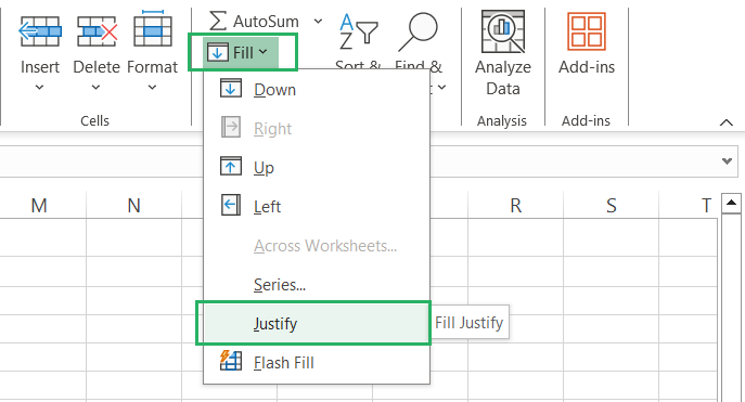
Step 2) is to go to the Home tab > Editing group > Fill button > Justify.

You’ll see all the rows will be combined into multiple rows such that they perfectly fit the column width.

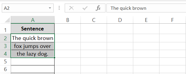
But we want them all combined in a single row.

Step 3) Adjust the width of the first column such that the entire sentence can fit into it.

Step 4) Again, select these three rows.

Step 5) Go to the Home tab > Editing group > Fill button > Justify Fill.

This time all these rows will be combined into one row.

Here’s something for you to note. The Justify fill feature combines all the selected rows into one with a space character between them. So, if you are collating a sentence like done in this example, this feature works the best for you 😎

However, if you want any other separator between each row, this feature might not prove to be the best for you.

The best method for this situation is using the functions that we are going to discuss next.

Combining Rows in Excel using CONCAT Function

The CONCAT function is available in Excel 2016 and later versions. It combines the contents of multiple cells into one 👌

Let’s try it here to see how it works.

Step 1) Choose the cell where you want the combined data to appear.

Step 2) Activate it and begin writing the CONCAT function as follows:

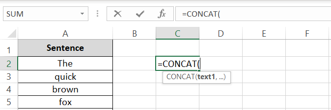
Step 3) Refer to the first cell that you want combined.

Step 4) In the next argument, add a space character enclosed in double quotation marks or any other separator (comma, dash, etc.) that you want between the combined cells.

Step 5) Then refer to the second cell that you want combined.

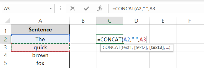
Step 6) Continue doing this for all the cells that you want to be combined until the CONCAT function looks like below.

Step 7) Hit Enter to see the results.

This method allows for combining both text and numeric data but does not automatically add delimiters (such as spaces or commas) between the combined values.

Hence, this method doesn’t suit situations like ours where you want a separator after each row.

It is better suited to the following situations where you want to combine data without any separators in between. In this case, you can refer to the range of rows at once instead of separately referring to each cell 🤔

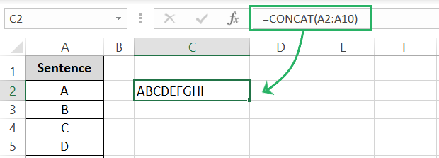
However, a plus point to using this and all merging functions is that they work dynamically. As you make any change to the original data in the cells, the combined data will change automatically.

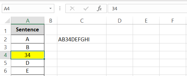
Look out for your situation to decide if this method suits you the best.

Combining Rows in Excel using the TEXTJOIN Function

The TEXTJOIN function is another function used to combine multiple cells in Excel. It is a much more advanced version of the CONCAT function 🙌

You can specify the delimiter to it for once and it will add it between each combined row. Let me show you here.

Step 1) Click on the cell where you want the combined data to appear.

Step 2) Type the TEXTJOIN function as below:

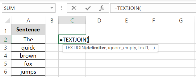
Step 3) Enter a space character enclosed in double quotation as the Delimiter Argument.

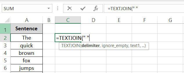
Step 4) Set the Ignore_Empty argument to TRUE.

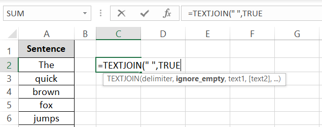
This argument specifies whether to ignore empty cells. TRUE means ignore empty cells; FALSE means include empty cells 🚀

Step 5) As the Text1 argument, specify the range of cells that you want combined. We will write this as A2:A10.

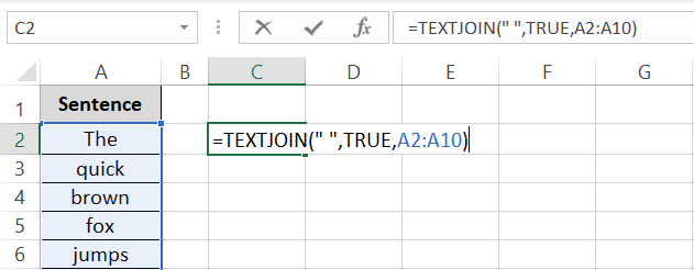
To join text from non-continuous cells, you can list them separated by commas, e.g., A1, A2, A3, A4, A5.

Step 6) Hit the Enter key to see what we get.

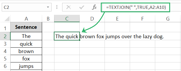
The contents of the specified cells are combined into one cell, with the specified delimiter in between each text item.

TEXTJOIN makes merging cells very convenient and quick. Perfect for situations where you want to combine multiple rows with a specified delimiter.

Combining Rows in Excel using the Ampersand Operator

An ampersand operator also merges cells and texts. It works the same as the CONCAT function, just that it is not a function but an operator ➕

Let’s combine the cells in our example using the ampersand and see how it turns out.

Step 1) Activate the cell where you want the combined data to appear.

Step 2) Begin writing the formula as follows:

Step 3) Add an ampersand operator.

Step 4) Add a space character as the separator.

Step 5) Add another ampersand operator and refer to the next cell to be combined.

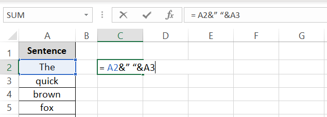
Step 6) Continue doing the same until all the cells are combined.

Step 7) Press Enter to see all the rows combined.

The contents of cells A2 to A10 will be combined into the selected cell with a space character in between 🧪

This method is even longer than the CONCAT function, you have to refer to each cell individually with an ampersand in between. Can’t refer to a cell range together.

Hence, it is not recommended if you have a long list of cells to combine.

Conclusion

Combining rows in Microsoft Excel can be done using various methods& each is suited for different scenarios and Excel versions.

In this guide, we have seen a great deal of such methods starting from Justify Fill and Ampersand operator to multiple functions like the CONCAT and TEXTJOIN functions.

The Fill Justify feature is great for quick text combinations& while the CONCAT and TEXTJOIN functions offer more flexibility and functionality. The Ampersand operator is a simple and universal solution.

Enjoyed checking out these methods? Then you’ll surely love the following Excel tutorials by Spreadsheeto that cover similarly amazing Excel tips. Check them out there.

• How to Combine Two Columns in Excel (No Data Loss)
• How to Combine First and Last Names in Excel (2024 Guide)
• How to Add Text to Excel Formula (Before& In& After)