How to Combine Two Columns in Excel (No Data Loss)

In Microsoft Excel, you can use the Merge Cells feature to combine two or more cells, columns, or rows.

This feature is best when you combine cells with no data in them. If these cells contain data, using the merge cells feature will cause you to lose some of it. 😬

So, is there any way you can combine data from two columns in Excel with no data loss?

Yes, there is! 👍

In this Excel tutorial, we’ll show you 2 main methods (and a bonus) on how to combine columns without losing any data.

Download this sample Excel workbook and let’s start.

Table of Contents

Merging Columns in Excel

When you want to merge columns in Excel, you can select the cells you want to combine and click the Merge & Center button in the Alignment group of the Home Tab. So easy!

If you merge cells with data, Microsoft Excel shows you this error message: “Merging cells only keeps the upper-left value and discards other values.”

This means that you’ll lose data in the process.

And we don’t want that to happen.

Method 1: Using the Ampersand Symbol (&)

One of the major methods how you can combine columns without losing data is using the Ampersand Symbol.

The Ampersand symbol (&) is a text operator in Excel that joins one or more text strings to produce a single piece of text.

Open your Excel workbook. Let’s say you want to merge the data in column A which contains first names and the data in Column B which contains last names.

You want to fill the third column (Column C) with the first and last names combined.

Here’s how to do that step by step. 👇

Step 1) Double-click cell C2 to put the cell in edit mode and type the equal sign (=) to start the formula.

Step 2) Click on the first cell. In our example, cell A2.

Step 3) Type the Ampersand symbol (&)

Step 4) Click on the second cell that contains the data you want to combine. In our example, it’s cell B2.

Step 5) Press Enter

Ta-da!

You’ve successfully combined two columns without losing any data. 😊

To make the names look more proper, we can add a separator between the first name and the last name. You can type a space inside the quotation marks (“ “)

Or you can copy this Excel formula below and paste it on the formula bar.

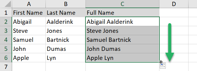
Fill in the next cells by double-clicking or dragging down the fill handle located at the bottom right corner of the cell.

Method 2: Using the CONCAT function

Another method how you can combine columns of data without any data loss is using the CONCAT function.

The CONCAT function is one of the text functions that allows you to join two or more text strings into one string.

The syntax of this function is =CONCAT(text1, [text2],…)

This function has the following arguments:

• text 1(required) – The first item to join. The item can be a text value, number, or cell reference.
• text2, … (optional) – Additional text items to be joined. There can be a maximum of 253 text arguments for the text items. Each can be a string, or array of strings, such as a range of cells.

Let’s try it.

Step 1) Double-click the cell and type =CONCAT(

Step 2) Click on the first cell. In our worksheet, select cell A2 and add a comma symbol (,)

Step 3) To add space between two text strings, type “ “ and a comma symbol (,)

Step 4) Click on the second cell. In our worksheet it’s cell B2. Close the function with a right parenthesis.

Step 5) Press Enter.

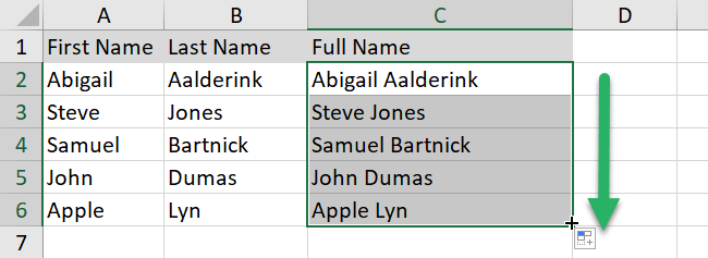
Fill in the next cells by double-clicking or dragging down the fill handle.

Bonus: Using Flash Fill

The fastest way to combine the data of two columns is Flash Fill. ⚡

Flash Fill is one of the most amazing Excel features as it automatically fills your data when it senses a pattern.

Using the data in our sample workbook, you can merge the data in first name and last name in a new column.

Step 1) Enter the full name in cell C2, and press ENTER.

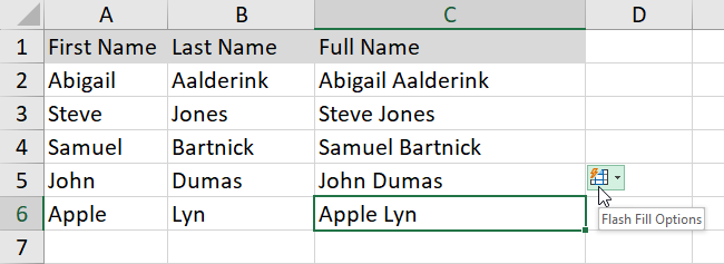
Step 2) Start typing the next full names, Excel will sense the pattern you provide, and show you a preview of the rest of the column filled in with your combined text.

Step 3) To accept the preview, press ENTER.

That’s it—Now What?

Good job! 🙌

You’ve learned how to combine data between two columns in Excel without any data loss in the process.

What’s next for you? Well, we have 300+ articles for you to learn more about the ins and outs of Microsoft Excel, and here are our top picks:

• How to Use TEXTJOIN in Excel: Concatenate Cells
• How to Make First Letter Capital in Excel: Step-by-Step
• How to Extract First Word in Excel in Less Than 1 Minute
• How to Remove Leading and Trailing Spaces in Excel