How to Switch First and Last Names in Excel (Easily)

Got a long list of names populated in Excel that looks like plain first and last names?

Do you want to switch the First Name and Last name in Excel? In a blink?

You are in the right place 📝

Switching first and last names in Excel can be done using several methods, each suited to different needs.

This guide will walk you through five different techniques to switch the first and last names in Excel. All you need to do is download the free practice workbook or this guide and slide below to learn them all.

Table of Contents

Switch First and Last Name in Excel through Flash Fill

Flash Fill is a powerful tool in Excel that automatically fills your data when it senses a pattern. And once I show you how to leverage this tool to switch the first and last names in Excel like a pro, you’ll love it too 🤩

Here I have a list of names in Excel.

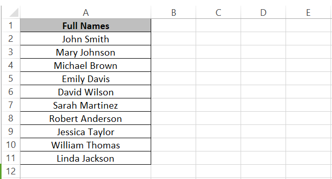
However, we want them written as “Last Name, First Name”. Let’s try the flash fill feature to see how this can be done.

Step 1) Activate a cell adjacent to the first row of names.

Step 2) Write in the name in the desired format i.e., “Last Name, First Name”.

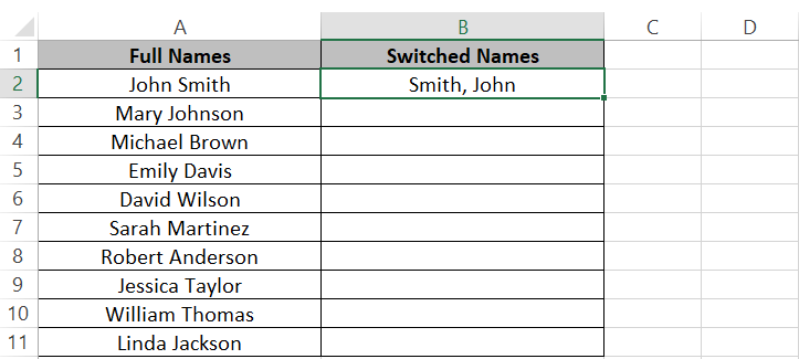
Step 3) Start typing the next switched name in the cell in the next row.

By now, Excel should recognize the pattern and suggest the remaining entries for switched names.

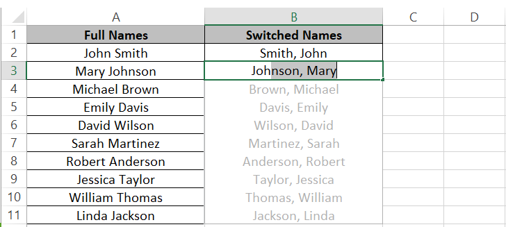
Step 4) Press Enter to accept the suggestions. Or, press the Ctrl + E key to trigger Flash Fill

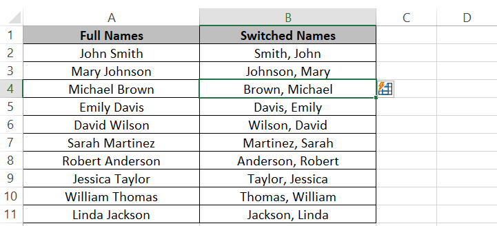
Excel would populate the remaining list until the last populated adjacent row based on the same pattern as defined above 🙌

Now you know why Flash Fill is one of my favorite features from Excel.

Switch Names through Excel Functions

You can also switch names in Excel by using a pair of functions. It is going to be a long formula with a couple of functions nested into it.

But the results are promising. If you have such data that keeps changing frequently, this method will suit you as these formulas capture the changes made to the original list of names.

Here’s what you need to do to switch names in Excel using functions 🥂

Step 1) Activate the first cell where you want the switch names.

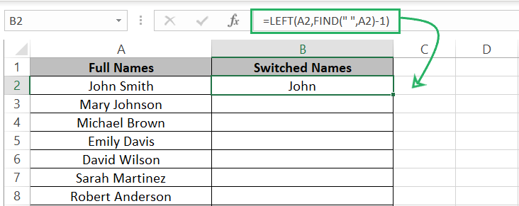
Step 2) Write the LEFT Function together with the FIND function as below to extract the first name from the names.

The LEFT function extracts a given number of text strings from the left side of a word.

• The first argument (A2) is the text from where the left strings are to be extracted.
• The second argument has to be the number of text strings to be extracted. We have replaced it with the FIND function that finds the space character from the text in Cell A2 and then deducts 1 from it.
• For Cell A2, the FIND function returns 5 (the space character comes at the 5th position), and then deducting 1 from it, we get 4. When nested into the LEFT function, we get the first 4 characters extracted from the word in Cell A2.

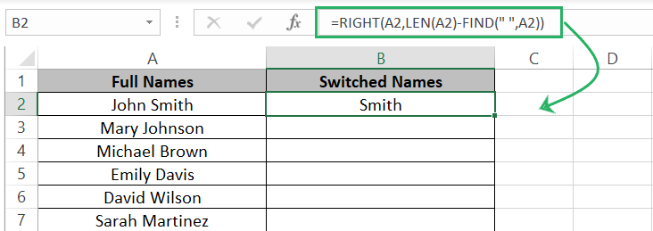
Step 3) Now write the RIGHT function together with the LEN and FIND function to extract the last name from Cell A2.

The RIGHT function extracts a given number of text strings from the right side of a word 💡

• The first argument (A2) is the text from where the strings on the right are to be extracted.
• The second argument has to be the number of text strings to be extracted. We have replaced it with the LEN function that returns the length of a given text string. From the length of the text string, we deduct the space character and the characters before it by using the FIND function [FIND(“ “,A2)].
• For Cell A2, the LEN function returns 10. From this, we deduct 5 (returned by the FIND function). When nested into the RIGHT function, we get the last 5 characters extracted from the word in Cell A2.

Now, as we have devised a formula to extract the first and the last names individually, all we need to do is concatenate these functions together.

Step 4) Concatenate both these functions together by nesting them into the CONCAT function as follows:

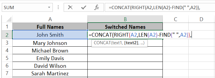
The function to extract the last name comes first.

Step 5) As the next argument, add a comma in double quotation marks (the separator between the last name and the first name).

Step 6) Then comes the function to extract the first name from the name.

Step 7) Press Enter.

Tada! The last and the first name is concatenated with a comma in between.

Step 8) Drag this formula down the whole list to have all the names switched.

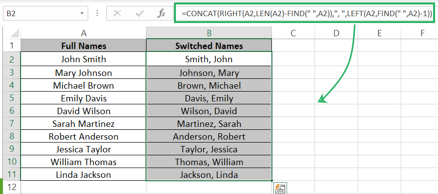
There you have it! We get the names in the “Last Name, First Name” format. The best part, if you make any change to the original names, the switched names will accordingly change 🚴‍♂️

Cool, isn’t it?

Switch Names through Text to Columns Feature

You must have heard of the Text to Columns Feature. It splits the text in a cell into multiple columns.

Want to see a demo? Let me show you here 😎

Step 1) Select the range of names.

Step 2) Go to the Data tab > Data Tools > Text to Columns.

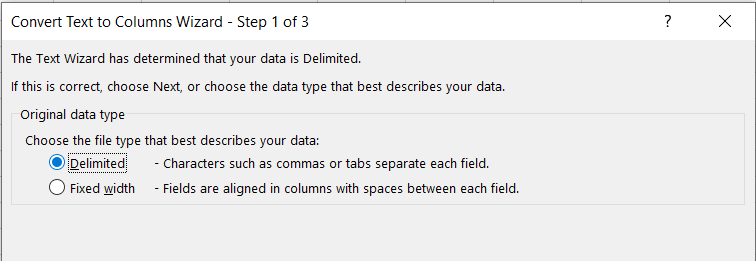
Step 3) In the Text to Columns Wizard, choose Delimited and click Next.

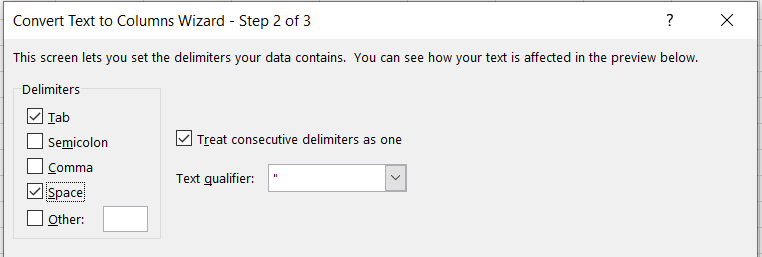
Step 4) Select Space as the delimiter and click Finish.

The column of names will now be split into two (a column for first names and a column for last names).

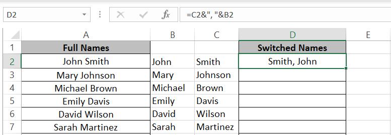
Step 5) Combine the last and the first name with a comma in between by using the ampersand operator as shown below.

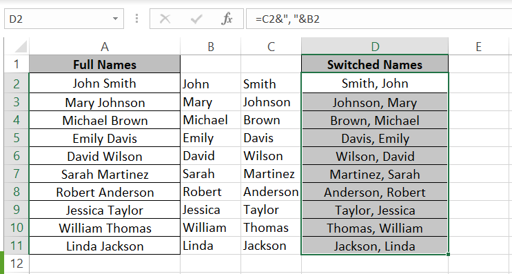
Step 6) Drag the fill handle down the whole list of names.

And that’s it. You get the names switched and arrange in the “Last name, first name” order.

Set up a Power Query to switch names

The Power Query method to switch names in Excel is a little longer and may be more complex than the previous methods.

However, if you have such data at your disposal frequently, you can save this query and re-run it again and again to save time ⏲

So, let’s try it out and see how you can switch first and last names in Excel by using the Power Query editor.

Step 1) Select the data range containing the names.

Step 2) Go to the Data tab > Get & Transform Data > From Table/Range.

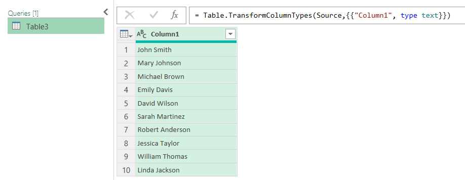
This will launch the Power Query Editor with the selected data loaded into it as below.

Step 3) Right-click on the header of this column and select Split Column > By Delimiter.

Step 4) In the Split Column by Delimiter window, select Space as the Delimiter (or if the names in your dataset are separated by any other character, select it as the delimiter).

Step 5) Click okay.

The column will now be split into two columns.

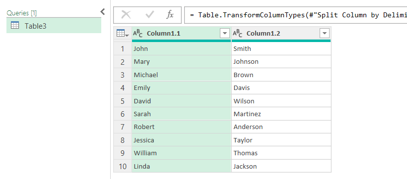
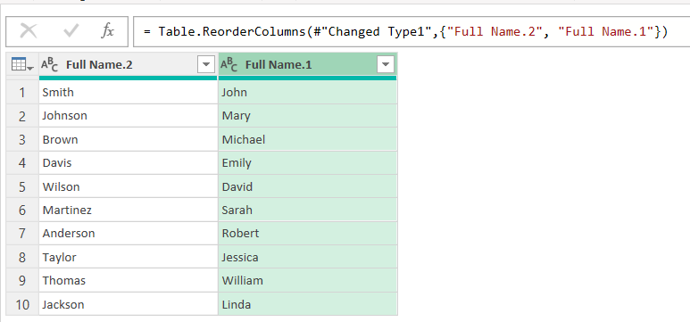
Step 6) Hold down the header for the column of first names and drag it towards the right.

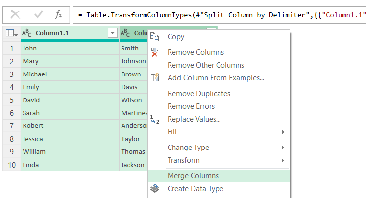
Step 7) Click on the header of the column for the last names, hold down the Ctrl key, and click on the header of the column for first names.

Step 8) Right-click to launch the context menu and select the option to Merge Columns.

Step 9) From the Merge Columns dialog box, select the Separator as Custom.

Step 10) Add a comma and a space character ( ,) as the separator.

Step 11) Set up the new column name as you want it.

Step 12) Click okay.

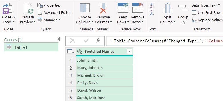
The names will be switched in the “Last name, first name” format as a merged column 🥽

Step 13) Click on the Close & Load button on the top right of the Power Query Editor.

You’ll see the new column of merged names will appear as a new sheet added to your workbook.

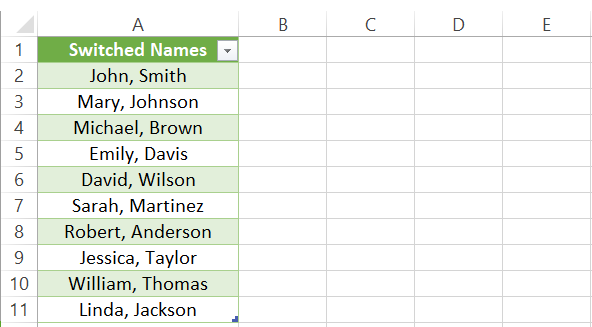
Again, it is not advised to use this method if you’re only looking to switch names in Excel. However, if this is something that you get to do often, setting up a Power Query for it can help you job in big time.

VBA Script to switch names

Lastly, you can also write a VBA code to switch names in Excel.

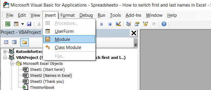
Step 1) Press the Alt key + F11 to open the VBA Editor.

Step 2) Go to the Insert tab > Module.

Step 3) In the Module window, copy and paste the following code.

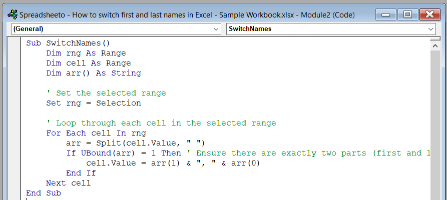
Step 4) Close the Module window and the VBA editor.

Step 5) Select the range of cells containing the names to be switched.

Step 6) Press the Alt + F8 key to launch the Macro dialog box.

Step 7) From the Macro dialog box, select the VBA code “SwitchNames” and click Run.

Excel will run the code and the names in the selected range will be switched with a comma in between 🎭

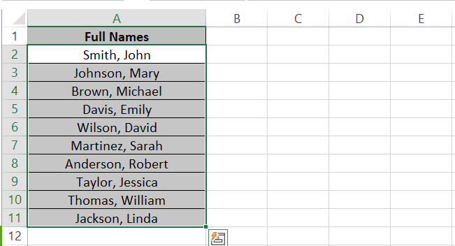
This method helps you to switch names placed anywhere in your sheet and they are switched in their place. For example, names placed in Column A are switched within Column A.

You do not need to create an extra column or displace the original names.

Conclusion

You can switch names in Excel and bring them to any format you like by using a variety of methods.

In the above guide, we have seen how you can leverage these methods to switch the first and last names in Excel. Starting from the easiest flash fill method, to using Excel functions, Text to Columns feature, Power query editor, and running a VBA script.

Choose the method that best fits your specific requirements and saves you the most time. To keep learning amazing things about Microsoft Excel, do give the following Spreadsheeto Excel tutorials a read.

• Text to Columns Guide: How to Separate Data in Excel
• How to Split Text in Formula (TEXTSPLIT Function)
• How to Split an Excel Cell (The Best Methods)