How to Count Unique Values in Excel (and Distinct Values)
Are you tired of manually counting the unique and distinct values in your Excel spreadsheet?
Don’t worry; there’s a much easier way!
In this guide, we’ll show you how to use Excel’s built-in functions to count unique and distinct values.
So let’s dive in and learn how to count unique values in Excel like a pro! 🥽
You can also download our sample workbook here if you want to practice along the guide.
Table of Contents
What do unique values really mean? (distinct values)
As the name suggests, unique values occur in a data set only once. Distinct values, on the other hand, are different from each other.
This means that while a unique value can occur only once in a data set, a distinct value may occur twice but will only be counted once 1️⃣
Let’s understand this through a demonstration below.
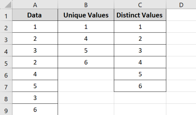
As evident from the image, unique values contain the numbers that only occur once in the data set. And distinct values contain numbers that are duplicated along with the unique values.
Unique or distinct values are often used in data analysis. By identifying these values, we can determine how many categories exist in the data set.
Let’s now see how to find unique and distinct values in a data set below.
Count UNIQUE values in Excel
To count unique values in our data set, we use a combination of the IF, SUM and COUNTIF functions. Applying the formula is very easy, and you will be able to master it in no time once you get a hold of it.
The general form of the formula to count unique values looks like this:
=SUM(IF(COUNTIF(range, range)=1,1,0))
Seems daunting, right? 😅
But don’t worry; we will go over each function in this formula in detail below.
Let’s now look at an example of counting unique values.
Say, we have the following sample data.

It contains a list of random numbers. We want to filter out all the unique values in the data set.
To do that,
- Select cell B2.
- Enter the IF and SUM function to count unique values as:
=SUM(IF(
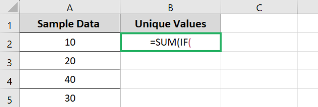
- Now add the COUNTIF function as:
=SUM(IF(COUNTIF(
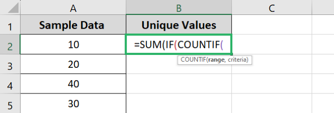
- Enter the range that contains unique values.
=SUM(IF(COUNTIF(A2:A10, A2:A10)
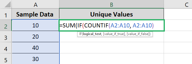
- Now add the values.
=SUM(IF(COUNTIF(A2:A10,A2:A10)=1,1,0))
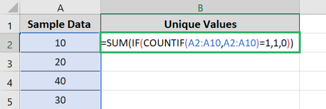
Note that this is an array formula. To get the result, press the keys CTRL + SHIFT + Enter on your keyboard. Doing this will automatically add braces to the formula and calculate it.
Excel returns the result as:
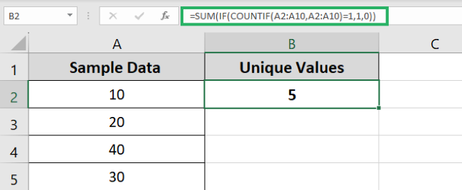
There are five unique values in our data set, as evident from the result.
Now let's break down this formula.
- The COUNTIF function shows the number of times a single value appears in a data set. For example, COUNTIF(A2:A10) would return . 1 represents unique values, whereas 2 represents duplicate values. For instance, 1 corresponds to 10 as it is a unique value.
Pro Tip!
You can check the array returned by COUNTIF function yourself. Simply select the function whose array you want to check in the formula bar and press F9. That portion of the function will be replaced with its array.
- IF function checks all the values returned by COUNTIF to be true. If the values are true or 1, the IF function returns 1. And if false, the IF function returns 0. So the above array becomes . Zero represents duplicate values.
- Lastly, the SUM function adds up the array obtained from the IF function. In this case, it will sum and return 5 – our desired answer.
See? It's really that simple. Trying it for the first time might seem difficult, but you will be a lot more proficient when you do it the second time 😉
Count DISTINCT values in Excel
There are two ways you can count distinct values in Excel. Both are tricky, but once you understand them, counting distinct values will be a breeze.
You can count distinct values by using a formula and by using a pivot table. Let’s see both methods below 😃
Count distinct with a formula
The formula to calculate distinct values is as follows:
=SUM(1/COUNTIF(range, range))
We can also use another variation of this formula with SUMPRODUCT as:
=SUMPRODUCT(1/COUNTIF(range, range))
We will use the same data set as seen earlier so we can better identify the difference.
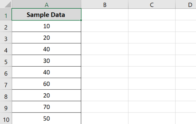
We want to find the count of distinct values in this data set. To do that,
- Select cell B2.
- Enter the formula as:
=SUM(
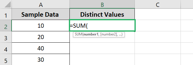
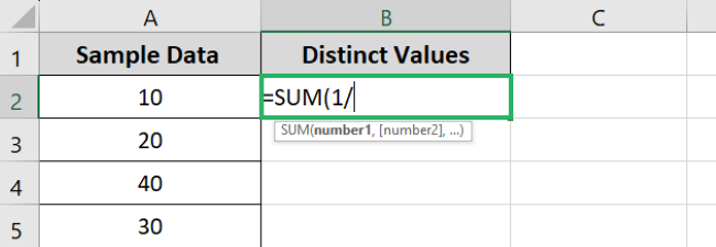
- Now apply the division operator.
=SUM(1/
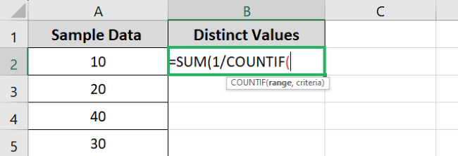
- Enter the COUNTIF function.
=SUM(1/COUNTIF(
- Select the range containing values.
=SUM(1/COUNTIF(A2:A10,A2:A10))
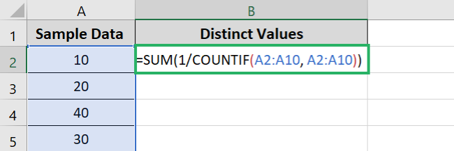
Remember to press CTRL + SHIFT + Enter on your keyboard, as this is an array formula.
Excel returns the result as:
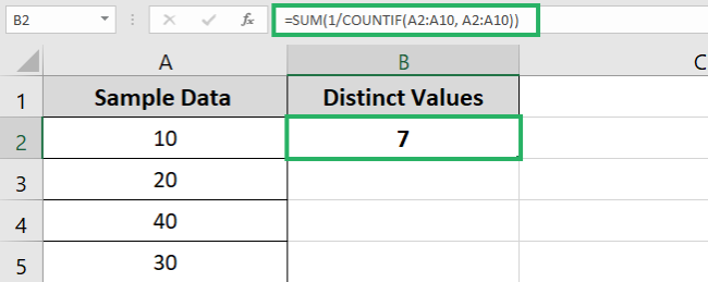
As visible, the result is seven. This shows there are seven distinct values in our data set.
Let's now break down the formula and look into each function separately 🔽
- The COUNTIF function returns the number of times an individual value occurs in the data set. In this example, COUNTIF returns the array .
- 1/COUNTIF divides the returned array by 1 and returns . Each duplicate value is converted to 0.5 (1/2=0.5).
- The SUM or SUMPRODUCT function adds up all the values in the final array and returns the expected result – 7.
Count distinct with a pivot table
Let's now explore how to count distinct values using a pivot table.
We will use the same data as used above.

To get the distinct count of our data set via a pivot table,
- Select the data set.
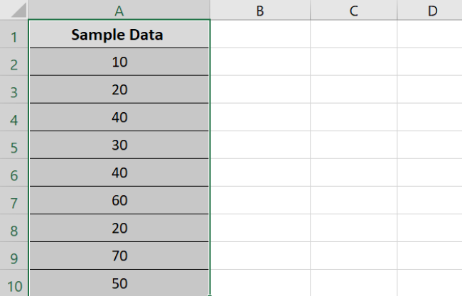
- Go to Insert Tab > Pivot Table.

- The Pivot table dialog box will appear.
- Select where you want to place the Pivot table. New worksheet is selected by default.
- Make sure to checkmark Add this data to the Data Model at the bottom of the dialog box.
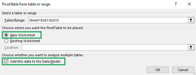
- Once the Pivot table appears, arrange it as you want. Creating your first pivot table? Learn everything you need to know about pivot tables in this step-by-step guide.
- Since our data set contains numbers, it will appear under the Values section by default. If not, simply move it there.
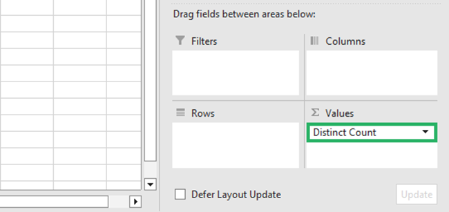
- Right-click the drop-down next to the name of the table – in our case – Distinct Values Count.
- A drop-down menu will appear.
- Click Value Field Settings.
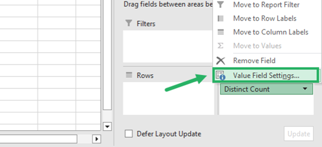
The Value Field Setting dialog box will appear.
- Scroll down under Summarize Value Field By and select Distinct Count.
- You can also change the name of your Pivot table by setting a custom name.
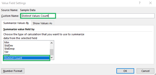
- Press Ok.
And voila! It’s done 🥇
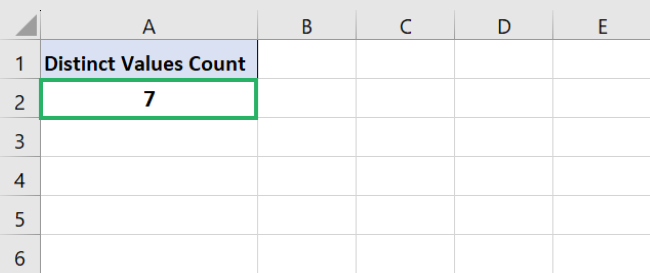
The Table will show the count of distinct values in the data set – 7.
It did take some time and concentration, but now that we have the count, it doesn’t seem too difficult, does it?
Practice it a couple of times, and you will have mastered it in no time 🎯
That’s it – Now what?
In this article, we saw how to count unique and distinct values in excel. We learned how to do it using a formula and a pivot table.
Counting unique and distinct values in Excel doesn’t have to be a daunting task.
By using Excel’s powerful functions, you can quickly find the number of unique values in your data 🤩
Excel also has a variety of other functions that are just resourceful. Some of these include IF, SUMIF and VLOOKUP, etc.
You can learn them for free in my 30-minute free email course that teaches this and a lot more. So don’t waste any more time manually counting values.
Other relevant resources
Did you enjoy reading this article? If yes, then you’d love to know more.
Read similar topics: COUNT function, COUNTIF function, Pivot Tables, and more.
