How to Use the CEILING Function in Excel – and Why!
Just like the name suggests – the CEILING functions rounds a number up🙈
How does it round the number up? And why use the CEILING function to round figures in Excel?
All of this and much more await you in the guide below. So download our free sample workbook right now and continue reading👇
Table of Contents
What to use the CEILING function for
The CEILING function is used to round numbers up to the nearest multiple of the number supplied as the significance. Must have sounded alien🤯
But let me explain this to you. Here’s how you write the CEILING function in Excel.
= CEILING (Number, significance)
- The number is the value that you want to be rounded up.
- Significance is the number whose multiple is used to round the number up.
For example, write the CEILING function as follows:
= CEILING (11,2)

To get the answer 12.

The CEILING function tells Excel to round the number 11 up to the nearest multiple of 2.
The two closest multiples of 2 around 11 are:
- 10
- 12
As the CEILING function rounds a number up (and not down), it returns 12😏
Hope that explains how the CEILING function works.
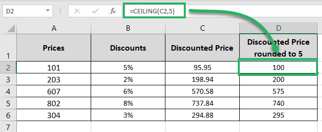
The CEILING function can be used in financial analysis. You can also set it to determine a rounded price after different currency conversions, a percentage discount, commissions, etc.
For example:
If you are offering discounts to different customers on a variety of items that are differently priced, you can use the CEILING function to get the discounted price as a round multiple of 5💪
Pro Tip!
What you must note is that the CEILING function only rounds up the numbers.
To similarly round down the numbers (based on the same science as the CEILING function), use the twin brother of the CEILING function i.e. the FLOOR function👨🏿🤝👨🏼
How to use the CEILING function
Using the CEILING function in Excel is simple. It takes two arguments only. Let’s write one to understand it better.
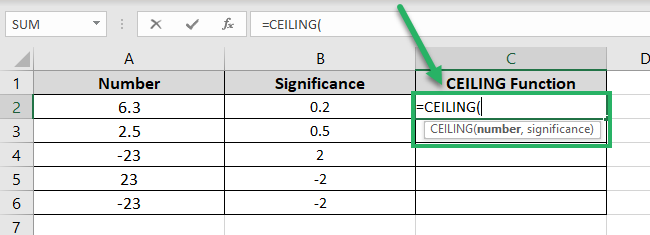
- Begin writing the CEILING function as follows:
= CEILING (
- As the number, refer to the cell containing the number to be rounded up. Or write that number in yourself.
= CEILING (A2
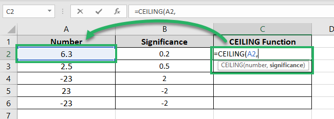
We have referred to Cell A2 as the number.
- The significance argument refers to the cell containing the number whose multiple is sought.
We are referring to Cell B2 here🪁
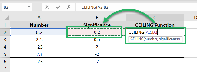
- Hit Enter to get the result as follows.
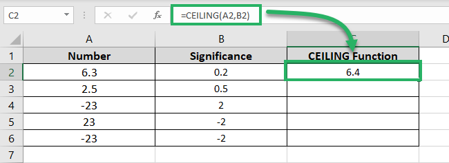
The answer is 6.4 as the closest two multiples of 0.2 near 6.3 are as follows:
- = 31 * 0.2 = 6.2
- = 32 * 0.2 = 6.4
And as the CEILING function will round the answer up, we get 6.4🥇
It must’ve been simple until now, but things get more interesting hereafter.
- Drag and drop the results to the whole list.
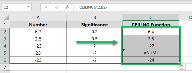
These results might raise some questions. Here are the answers.
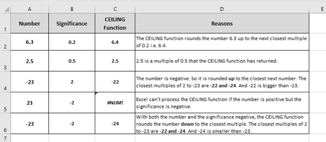
Pro Tip!
Until Excel 2007, the CEILING function couldn’t process negative arguments❌
But, in the 2010 and latest versions of Excel, the following combinations of positive/negative numbers and significance can result as follows:
| Number | Significance | CEILING Function |
|---|---|---|
| Positive | Positive | Rounds up to the next positive multiple |
| Negative | Positive | Rounds up to the next negative multiple |
| Positive | Negative | Error |
| Negative | Negative | Rounds down to the next negative multiple |
That’s it – Now what?
Here we come to the end of this guide. In the guide above, we have learned all about using the CEILING function in Excel. What can you use it for, and how do you use it?
Using this smart function, you can bring all numbers in your Excel sheet to symmetry. But that’s only one function of Excel. The variety of other similar useful functions to be offered by Microsoft Excel is so vast to be explored😎
Some of my favorite Excel functions include the VLOOKUP, SUMIF, and IF functions. They are too smart to let go.
Other resources
The CEILING function is not the only way to round figures in Excel.
