How to Round Up in Excel (or Down) – 2024 Full Guide

Rounding numbers is a way of simplifying numbers to make them easier to understand or work with. Although by rounding, you only get an estimated value that is still relatively close to the exact value. 😊

But what if you need to round numbers to a specified number of digits ONLY? How do you eliminate the least significant digits then? How do you set it with only 2 or 3 digits after the decimal point? 😱

Well, Excel got these Rounding functions to help you. The ROUNDUP, ROUNDDOWN, and ROUND functions.

Are you ready for a round of rounding numbers? 💪 Download your practice workbook here.

How to round up numbers in Excel

The ROUNDUP function in Excel is used to round a number up to its nearest integer, away from 0 (zero).

The syntax of the ROUNDUP function is =ROUNDUP(number, num_digits).

This function has the following arguments:

1. Number – Any real number you want to round up.
2. Num_digits – The number of digits to which you want to round the number to.

Let’s go! ROUND 1. 🥊

Let’s use the value of pi (π = 3.14159265359) for our example.

Here’s how to round up this number to your desired number of digits.

1. In cell B2, type =ROUNDUP(

2. The first argument of the ROUNDUP function is the number. Type the number or click on the cell address of the number you want to round up.

=ROUNDUP(A2,

3. The next argument is num_digits. It is the number of digits you want to round the number to.

Let’s use 1 for our first example. 1 means to round a number to one decimal place after the decimal point.

Simply put, round to the nearest tenths. Close the function with a right parenthesis.

=ROUNDUP(A2,1)

4. Press Enter.

The number ROUNDED UP.

Since the num_digits is 1, the number is rounded up to the nearest tenths (the first decimal place to the right after the decimal point).

1 being the tenths decimal place value rounds up to 2, resulting to 3.2

Great job! 👍

Let’s try to input 2 as our num_digits. This means that the number rounds up to two decimal places (round to the nearest hundredths).

In cell B3, type =ROUNDUP(A3,2)

Press Enter.

The number is now rounded up to two decimal places. The hundredths decimal place rounds up to 5, resulting to 3.15

What a good starting ROUND! 🙌

Important to Note:

• If the num_digits is greater than 0 (zero), then the number is rounded up to that specified number of decimal places.
• The number to the right of the rounding digit doesn’t matter if it is below 5 or above 5 (Math rules in Rounding). It always ROUNDS UP to the nearest integer.

Ready for ROUND 2? 💪

Round up to the nearest whole number

To round a number to the nearest whole is very easy. 👌

Just apply the rounding formula used above and set the num_digits in the ROUNDUP function to 0 (zero).

In your practice workbook, you’ll see random numbers in decimal values. Decimal values or numbers consist of a whole number and fractional parts separated by a decimal point.

Let’s round up these numbers to their nearest whole.

1. In cell B2, type the ROUNDUP function:

=ROUNDUP(

2. The first argument in the ROUNDUP function is number. Type A2 or click cell A2.

=ROUNDUP(A2,

3. The next argument in the ROUNDUP function is num_digits. To round a number to its nearest whole number, type 0 (zero) for your num_digits.

=ROUNDUP(A2,0)

4. Press Enter. Fill in the next cells by double-clicking or dragging down the fill handle.

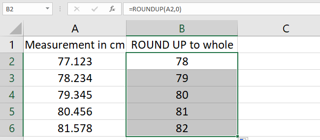
This is now the result.

Typing 0 (zero) as the num_digits in the ROUNDUP function rounds a number up to its nearest whole. It eliminated the decimal values.

The numbers after the decimal point DO NOT affect the rounding digits. Whether it’s less than 5 or more than 5, all are ROUNDED UP into their whole number. 👍

Round down

The ROUNDDOWN function is used to round numbers down to their nearest integer, towards zero (0).

The syntax of the ROUNDDOWN function is =ROUNDDOWN(number, num_digits).

This function has the following arguments:

1. Number – Any real number you want to be rounded down.
2. Num_digits – The number of digits to which you want to round the number to.

Let’s use the pi (π = 3.14159265359) example again.

1. In cell C2, type =ROUNDDOWN(

2. The first argument for the ROUNDDOWN function is the number. Click cell A2.

=ROUNDDOWN(A2,

3. The second argument for the ROUNDDOWN function is the num_digits. Type 1 for the num_digits.

=ROUNDDOWN(A2,1)

4. Press Enter.

This is the rounded number. It rounded down to one decimal place from 3.14159265359 to 3.1

What if we round down to two decimal places? ✌️

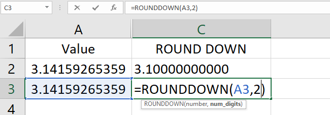
Type =ROUNDDOWN(A3,2)

Press Enter.

The number is rounded down to two decimal places (3.14) eliminating other digits.

Are you still DOWN for another round? 😊

Round to 2 decimal places

The ROUND function in Excel should not be confused with the ROUNDUP function.

The ROUND function rounds numbers to a specified number of digits following the Mathematics rules in rounding numbers. Do you still recall the rules?

Math Recall Class👨‍🏫

Rules for rounding numbers:

• The number to the right of the rounding digit will determine whether it will be rounded up or rounded down.
• If the number to the right of the rounding digit is 0 to 4, the rounding digit will not change, and the number will be rounded down.
• If the number to the right of the rounding digit is 5 to 9, the rounding digit will be increased by 1 (one), and the number will be rounded up.

The syntax of the ROUND function is =ROUND(number, num_digits) with the following arguments:

1. Number – Any real number you want to round.
2. Num_digits – The number of digits to which you want to round the number argument.

Let’s use the numbers in our workbook.

1. In cell C2, type =ROUND(

2. The first argument of the ROUND function is the number. Click cell A2.

=ROUND(A2,

3. The second argument of the ROUND function is the num_digits. Since we want to round the number to two decimal places, type 2 for the num_digits.

=ROUND(A2,2)

4. Press Enter. Fill in the remaining cells by double-clicking or dragging down the fill handle.

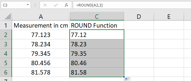
Now, you can see that all the numbers have 2 decimal places! The roundup or down was based on the third decimal place value.

When it is below 5, the rounding digit did not change, and the number is rounded down.

When it was 5 and above, the rounding digit is increased by 1, and the number rounded up.

The ROUND function follows the rules for rounding numbers.

You deserve a ROUND of applause! 👏👏👏

Round up to the nearest 10

To round up a number to the nearest 10, the CEILING function in Excel is what you’re going to use. The CEILING function in Excel rounds a number up to the nearest multiple of significance.

The syntax of the CEILING function is =CEILING(number, significance) with the following arguments:

1. Number – The value you want to round.
2. Significance – The multiple you want to round to.

Let’s try to round up 3.14159 to the nearest 10.

1. In a new sheet, type the CEILING function in cell B2.

=CEILING(

2. The first argument of the CEILING function is the number. Type in 3.14159 or click on cell A1.

=CEILING(A1,

3. The second argument of the CEILING function is the significance. The goal is to round up to the nearest 10. Input 10 as the significance.

=CEILING(A1,10)

4. Press Enter.

The number 3.14159 rounded to the nearest 10.

Remember that the significance can be any multiples you want to round a number to. It may be 2, 5, 10, or 100.

That’s it – Now what?

Congratulations! 🥳You have been victorious in all of the ROUNDS.

You now know your way through Excel’s ROUNDUP, ROUNDDOWN, and ROUND functions. The CEILING function was just a bonus!

Now, this may seem like a lot but these are a small selection of the helpful functions Excel has in store for you! 🤯

Some of the best ones are IF, SUMIF, and VLOOKUP.

You learn those in my free 30-minute Excel course.

Click here to read more about it (and enroll)🚀

Other resources

If you’re not looking to round a number but to shorten it, Excel’s TRUNC function is what you’re looking for!

If you’re into rounding, you might also be into making your spreadsheet easier on the eyes in general. For that, you can use conditional formatting, the format painter, and especially number formatting.