How to Expand All Columns in Excel At Once (Easy)

The easiest but often the most important part of your spreadsheet tasks is resizing column widths.

Whether you received a workbook with narrow columns all over it or you see clipped text in your worksheet, you know you need to fix the column widths 🔧

There are multiple ways to achieve the same result – some tedious while others efficient. In this tutorial, we will see all these methods in detail.

Before we begin, download our sample workbook below to practice along the guide. Let’s get right into it.

Table of Contents

Expand columns by dragging

The most obvious way of expanding columns in your MS Excel worksheet is to drag them using their double-headed arrow to your desired length 🧵

The problem with this method is that it’s rather unprofessional and gets very tiring. Imagine you have to resize a hundred columns by dragging them. Doesn’t sound cool, does it?

But if you’re a beginner or only have a couple of columns to deal with, this method might be a good choice 😉

Say, for instance, we have the following sample data with large text strings that don’t fit in the column. We want to resize the column according to the largest string it holds.

To do that,

Step 1) Hover over your desired column header to be resized.

Step 2) A double-headed arrow will appear at the column intersection.

Step 3) Click on the right edge of the column and drag it to expand to fit the largest string.

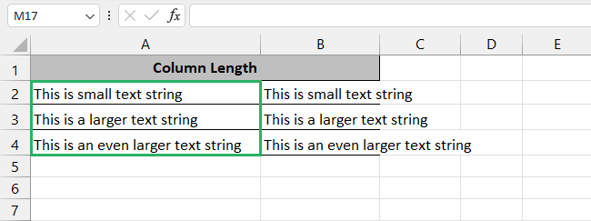
Step 4) That gets the entire column resized.

Step 5) Now, repeat the same process for the remaining columns.

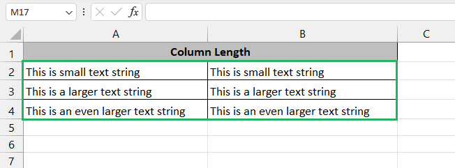
And it’s done!

It takes time but gets the work done 🤓

Expand columns by double-clicking

Another relatively more efficient way of resizing your columns is to use the double-click technique.

Say, we have the following sample data and we want to autofit the width of each column according to its largest string in one go.

To do that,

Step 1) Press CTRL + A or click on the box at the top left corner of the sheet where the row and column intersect to select the entire sheet.

Step 2) Hover over any column until the double-headed arrow appears.

Step 3) Double-click that column heading to expand the width of all columns in one go.

And ta-da! All columns in your sheet have been resized as per their largest string and it took less than 2 seconds.

This approach is more commonly used when working with files containing large data sets owing to its ease of use. Try it now! 😃

Expand columns using right-click menu

Another method you can use to expand columns is to use the right-click menu. It returns the same results but with a bit of extra flair. It gives you the option to specify the width of columns as you expand them.

In this method, the width of the columns won’t be dependent on the length of the largest string any longer, instead, the width of each column will be the same.

Let’s see how to do it below 🔽

Say, we have the following data set and I want to set the width of each column the same so that they look identical.

To do that,

Step 1) Select the columns you want to expand or press CTRL + A to select multiple columns in one go.

Step 2) Once done, right-click any column header.

Step 3) A drop-down list will appear.

Step 4) Select Column Width from the options.

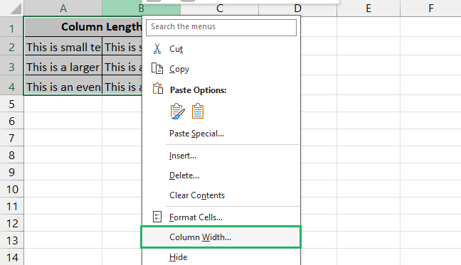
Step 5) A small dialogue box will appear on the screen.

Step 6) In the dialogue box, enter your desired width.

Step 7) Press Ok.

Voila! All columns have been set to the specified width. How cool is that? 😎

Pro-Tip

As wonderful as specifying column width sounds, it has a minor drawback. When you select all the columns in your Excel sheet, you are also selecting any columns that might be hidden.

In this case, when you set a particular width for all columns, the hidden columns will become unhidden and will appear on the sheet.

This is because a hidden cell essentially refers to the one whose column width is zero. So when setting a custom width for your column, make sure to double-check on whether you want to unhide those columns or not.

Expand columns using the Format menu

Next, we see how you can expand your columns using the Format menu through the ribbon 🎗

This method is more elaborate and commonly used because, unlike other methods, the Format menu offers two options you can apply to your Excel cells.

You can choose to autofit them according to their length or you can specify their width. Let’s now see an example of how this works.

Say, we have the following sample data in our Excel spreadsheet, and we want to expand them automatically 💻

To do that,

Step 1) Press CTRL + A to select the columns you want to resize or select them manually.

Step 2) Go to the Home tab 🏠

Step 3) Click on Format under the Cells section on the ribbon.

Step 4) Select AutoFit Column Width from the context menu.

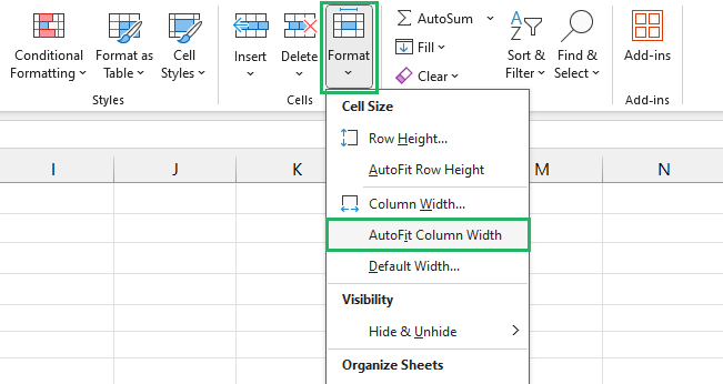
All the selected columns will be resized automatically according to their cell size.

If you were to set a specific width for the columns, do this,

Step 5) Click on the Format option 🎨

Step 6) Select Column Width from the menu.

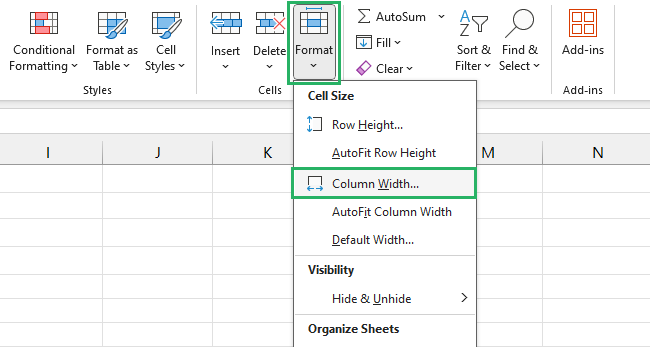
Step 7) A small dialog box will appear on the screen.

Step 8) In the dialogue box, enter your desired width.

Step 9) Press Ok.

And it’s done!

How simple was that 🧐

Expand columns using the keyboard shortcut

The quickest way to autofit columns in your sheet is to use a keyboard shortcut. It takes less than five seconds and all the columns in your sheet are resized instantly.

The use of keys in this shortcut makes it the optimal choice for Excel users who prefer sticking to their keyboards ⌨

Say, we have the following sample data to be resized according to its cell size.

To do that,

Step 1) Select the entire sheet by pressing CTRL + A or hold CTRL to select multiple columns.

Step 2) Press Alt key – this will open the key shortcut to accessing your ribbon.

Step 3) Right after that, press H – this would direct Excel to choose the Home tab.

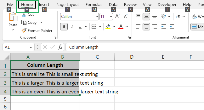
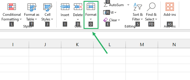
Step 4) Now, press O – this will take you to the Format option under the Cell section.

Step 5) Lastly, press I, this will select the AutoFit Column Width option from the dropdown menu.

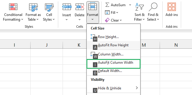
If you want to set a specific width, press W instead of I at the last step, it will then prompt you to enter the figure and it’s done.

So, the shortcut looks something like Alt + H + O + I on a whole. Pretty cool, no? 😃

Conclusion

In this Microsoft Excel tutorial, we saw how to expand columns in one go. We saw different methods including dragging and double-clicking autofit to adjust the width automatically.

To set a specific width, we saw the right click and Format option that lets you set the width as desired. Expanding columns is an essential trick you need to know to master Excel.

To learn more about columns and rows in Excel, read the below articles 📑

How to Make Cells Bigger in Excel (Width & Row Height)

How to Adjust Column Width in Excel: Step-by-Step (2024)

We hope you enjoyed reading this as much as we did creating it 🤗