How to Hide Formulas in Excel (But Still Show Data)

There are many situations why you may need to hide formulas in your Excel worksheets. 👀

For example, when you’re sharing Excel files with other users, and you don’t want them to edit or change anything important especially the formulas in the sheets.

Or when you’re sending Excel files, you may want others to see the final values but you don’t want them to know how these values are calculated.

Whatever the reason, learning how to hide formulas in Excel is important. 👍

It’s a straightforward process and we’ll show you how to do it in this Excel tutorial. To start, download this Excel workbook we’ve created for you.

Table of Contents

Hide ALL Formulas in Excel

There are two ways to see the formulas in the cells of your Excel worksheet:

Step 1) Select the cell and see the formula in the formula bar, or

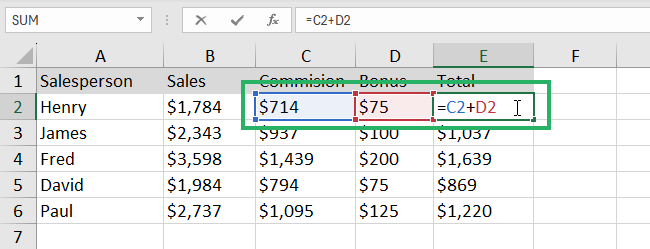
Step 2) Double-click the cell to put the cell in edit mode.

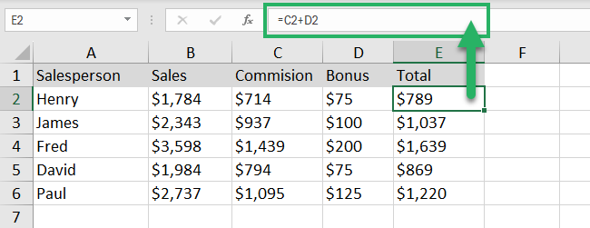
Open the sample Excel workbook. When you click cell E2, you’ll see the formula in the formula bar.

To hide formulas in Excel, 👇

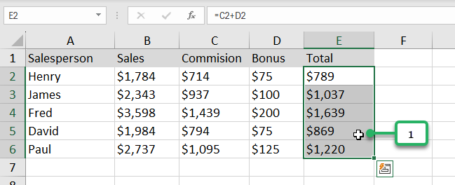
Step 1) Select the cells with formulas that you want to hide.

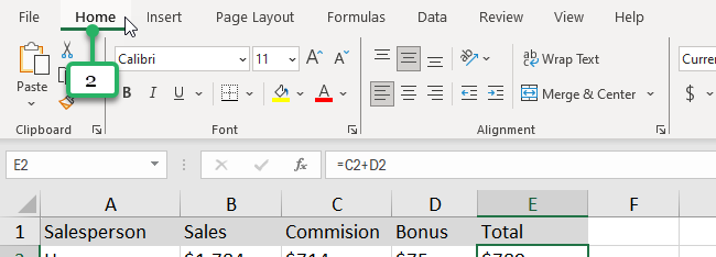
Step 2) Go to the Home Tab.

Step 3) In the Number group, click on the dialog box launcher. This will open the Format Cells dialog box.

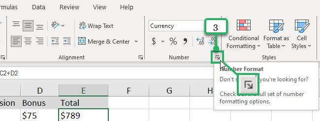
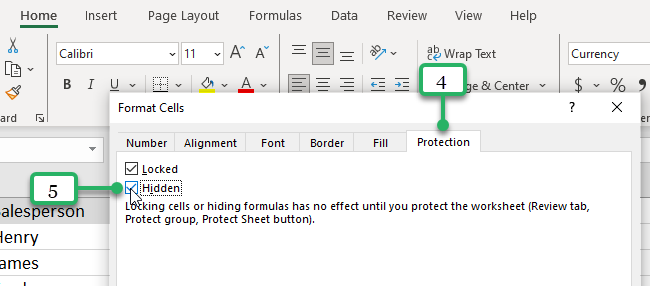
Step 4) In the Format Cells dialog box, click the Protection tab.

Step 5) Check the Hidden box.

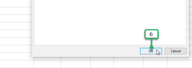
Step 6) Click OK.

In Microsoft Excel, hiding formulas has no effect yet until you protect the entire Excel worksheet. 🔒

Let’s continue.

Step 7) Go to the Review Tab.

Step 8) In the Protect group, click on the Protect Sheet button.

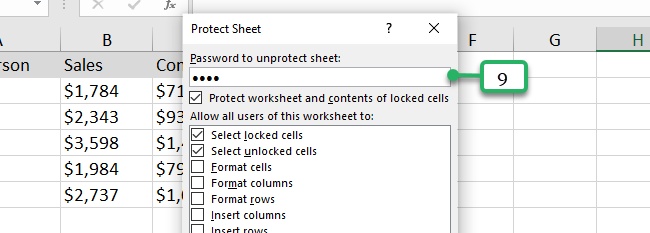
Step 9) In the Protection dialog box, enter the password that would be needed if you want to unlock the worksheet. In this example, you can type 1234.

Step 10) Finally, click OK.

You will need to confirm the password. So, type in 1234 again, and click OK to confirm.

The steps above have protected your entire worksheet in a way that your formulas are hidden.

Now, if you click on the cell that contains a formula, no formula is shown in the formula bar.

If in any case, a user tries to double-click on the cells to edit the formulas, Microsoft Excel shows this error message.

When other users want to change anything in the worksheet, they may need to ask for the password from you.

This will give your worksheet extra protection without anyone editing or overwriting any important formulas. Be it intentionally or accidentally. 👍

Hide Formulas in Excel (But Still Allow Input)

In the tutorial above, we’ve shown you how you can protect your entire worksheet. This protects both the cells with and without any formulas in it.

If you only want to hide formulas and keep the other parts of your worksheet editable, that’s possible too.

This allows other users to input data while you make sure the formulas are still intact.

Step 1 – Unprotect the Worksheet

Since we’ve previously protected the sheet in our Excel workbook, we need to unprotect it to make any changes. To do that,

Step 1.1) Go to the Review Tab.

Step 1.2) In the Protect group, click on the Unprotect Sheet button.

Step 1.3) To unprotect the sheet, type in the password we’ve made. In this case, 1234.

Step 1.4) Click OK.

Step 2 – Disable the Lock Property for all the Cells

By default, MS Excel locks all the cells. So we need to unlock it first to make any changes.

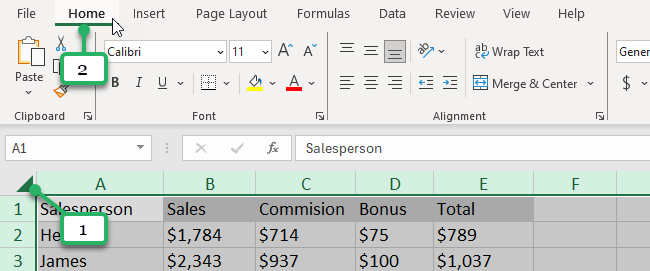
Step 2.1) Select all the cells in the worksheet by clicking the triangle on the top left corner of your worksheet area. You can also press Ctrl + A.

Step 2.2) Go to the Home Tab.

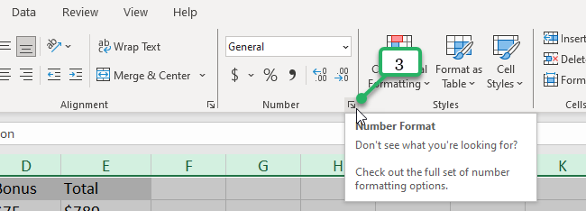
Step 2.3) In the Number group, click on the dialog box launcher. This will open the Format Cells dialog box.

Step 2.4) In the Format Cells dialog box, click the Protection tab.

Step 2.5) Uncheck the Locked checkbox.

Step 2.6) Uncheck the Hidden checkbox.

Step 2.7) Click OK.

Step 3 – Enable the Locked and Hidden Property Selected Cells with Formulas

Now we only need to identify the cells with formulas so we can lock and hide them.

Step 3.1) Go to the Home Tab.

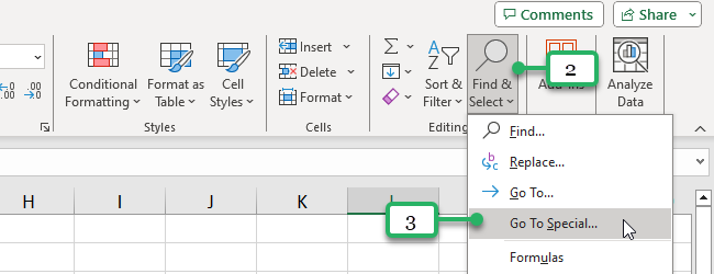
Step 3.2) In the Editing group, click the Find and Select button.

Step 3.3) Select the Go To Special option from the drop-down. This will open the Go To Special dialog box.

Step 3.4) Click Formulas.

Step 3.5) Click OK.

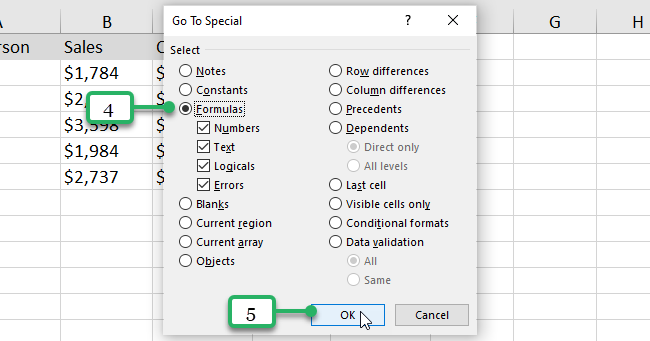
This selects all the cells with formulas in the worksheet.

Step 3.6) While the cells are selected, press Ctrl + 1 on your keyboard. This will open the Format Cells dialog box.

Step 3.7) Click on the Protection Tab.

Step 3.8) Click on the Locked checkbox.

Step 3.9) Click on the Hidden checkbox.

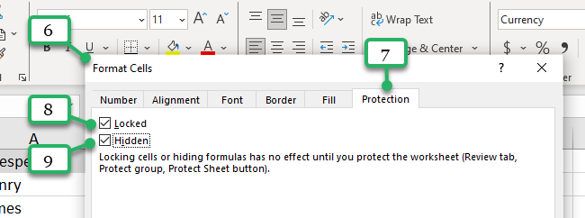
Step 3.10) Click OK.

Step 4 – Protect the Worksheet

To make the changes in full effect, we need to protect the worksheet.

Step 4.1) Go to the Review Tab.

Step 4.2) In the Protect group, click on the Protect Sheet button.

Step 4.3) In the Protection dialog box, enter the password that would be needed if you want to unlock the worksheet. In this example, you can type 1234.

Step 4.4) Finally, click OK.

You will need to confirm the password. So, type in 1234 again, and click OK to confirm.

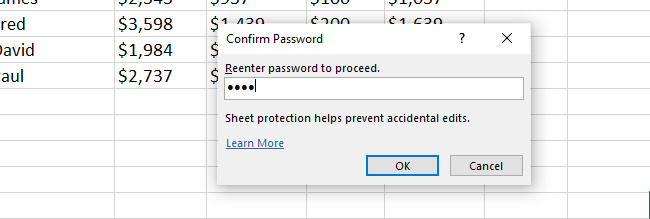
You can check that the rest of the cells are editable but the cells with formulas are locked and hidden. That means other users can’t edit these cells and their formulas are not shown in the formula bar. 🔍

That’s it—Now What?

Awesome! 🚀

Learning how to hide Excel formulas in your worksheets gives more control over what you want other Excel users to see and do in your worksheets.

In case you’re wondering what else can you hide in your Excel worksheets, then these related articles are for you:

• How to Hide Sheets in Excel: Step-by-Step (+ Superhiding)
• How to Hide and Show Excel’s Formula Bar (Instantly)
• How to Hide Filter Buttons in Excel in 1 Minute
• How to Lock Cells in Excel: Excel Protection Tutorial