How to Hide Filter Buttons in Excel in 1 minute
While working on a large data set in Excel, you add filter arrows to easily filter data.
To maintain your data set and make it more understandable for other Excel users, you may want to hide AutoFilter arrows.
It’s super quick and easy 😀
In this article, we’ll show you how to hide and show your filter buttons in Excel.
Table of Contents
Hide filter buttons
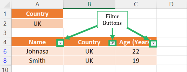
Each column header in the table below has a drop-down arrow 🔽
It was filtering the data range based on the country – the UK.
Therefore, you can see a filter icon on the country column heading (Column B).
The Excel sheet only displays filtered rows.
You may wish to hide Excel AutoFilter arrows for a variety of reasons.
For example, to keep your data table simple, to avoid mistakenly removing filters, and so on.
What happens if the table’s filtering buttons are removed? 🤔
The filtering settings will be deleted 😟
Therefore, while filtering your data range, how can each filter drop-down list be hidden?
To hide filter arrows in a filtered range, simply follow the instructions listed below 😍
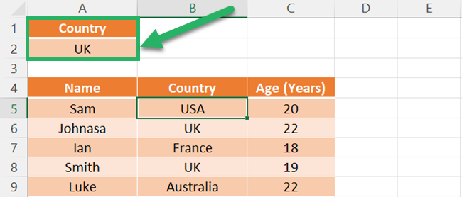
- Create a criteria values table with the same column headers.
So you can filter based on that list.
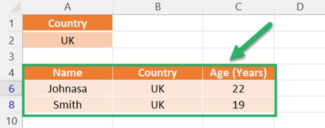
In the previous example, there is a separate table with the column header “Country” and the criteria “UK”.
You can use wildcard characters such as a question mark for a single character for text filters.
Also, logical operators for numeric data filters 🥳
- Go to the Data Tab.

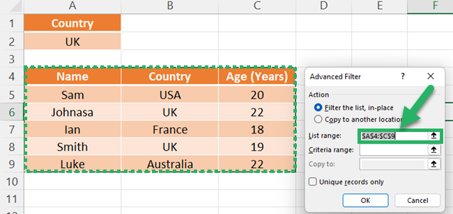
- Click the Advanced Filter button from the Sort & Filter group.

- Select your data table range as the List Range.
- Then, enter the criteria range. For this, you have to select the filter criteria table range.
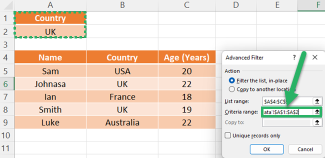
- Click the “OK” button.
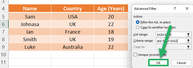
So, text values of the UK are filtered from the “country column in the above example without filter arrow buttons.
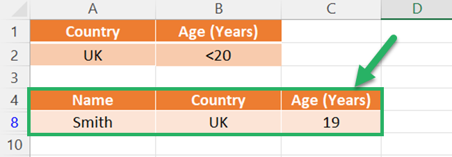
You can even create a filtering range with multiple criteria of many columns.
For example, you can expand your criteria values as shown below if you wish to select names from the UK, and who are under 20 years old.
Display filter buttons
If you want to display filter buttons on the header row of your table, you have to follow the below steps.
- Select a cell on your data range.
- Click the Filter icon using one of the following methods.
-
- Home Tab > Editing Group > Expand Sort & Filter > Filter
- Data Tab > Sort & Filter Group > Filter
- Press “Control + Shift + L”
- Expand the drop-down arrows and search values in the search box of the filter interface.
- The table will show only the information on custom filter data.
Pro Tip:
Let’s say that you want to filter the names of UK students in the above example.
You can easily filter that using the below steps.
- You can select a cell with the word UK from your data range.
- Right Click and go to the Filter
- Then, select “Filter by selected cell’s value”
You can easily apply text filters like that.
Then all other rows that do not equal the criteria will be hidden 🤩
That’s it – Now what?
Nice going! 👍
Knowing how to hide the filter buttons of your Excel tables will prevent other users from removing your filter settings so you can maintain your data table.
You can also hide AutoFilter arrows using Macros.
But that’s not only what Macros can do for you. Macros can help you do 50 things with a single click! 🤯
Sounds awesome?
Get started with Macros today with my free 30-minute online course where you’ll learn how to record and write a macro (and more!) ✍
Learn Excel the way you want–simple, quick, and practical😊
Other resources
This lesson is only a part of Excel data filtering.
To learn more about Excel filtering read our article – Full step-by-step guide for Excel Filters.
