How to Add a Filter in Excel (Step-by-Step)
Working with large datasets in Excel can make it hard to find relevant information.
The filter tool offered by Microsoft Excel makes it easy for users to narrow down their data to find what’s relevant.
To learn more about the filter tool of Excel (both basic and advanced), jump right into the article below.
Also, as you scroll down, download our sample workbook for free here.
Table of Contents
How to filter in Excel
The filter tool of Excel is a quick way to filter out the desired information only.
For example, the image below contains the sale data for some products.
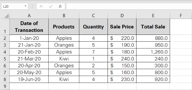
1. Apply filters to this data by selecting the header of the column where the filter is to be applied.
2. For example, if you want to filter sales based on product name, select the header for products.
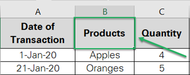
3. Go to the Data Tab > Sort & Filter > Filter.

Pro Tip!
There are two alternate shortcuts that you can use to apply filters to your data.
- Go to Home > Editing Group > Sort & Filter > Filter
- Use the keyboard shortcut to add filters – Control Key + Shift + L
4. This adds drop-down arrows to the selected column header (Products in this case).

5. The filter is already applied, and you can now use it to filter our information as desired.
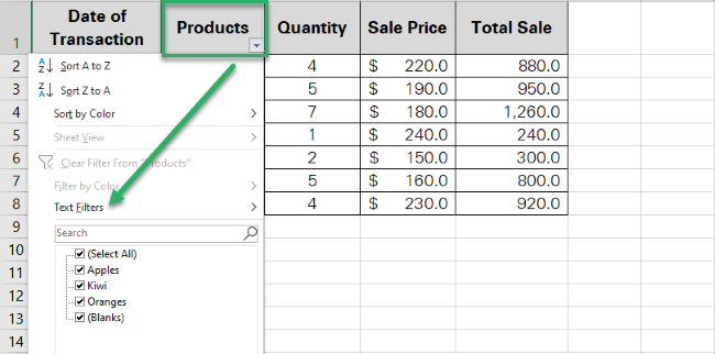
Must note that to apply filters, your data must have a proper column header where the filter is to be applied.
Using the filter tool, you can apply filters based on numeric or text values, format, or by criteria.
How to filter by text
Can you quickly filter out the sales of Apples made during the period❓
Simple. From the list of products, filter out the text ‘Apples’. The sales of Apples would be automatically filtered.
1. Apply filters to the column of products as explained above.
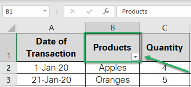
2. Click on the drop-down menu to launch the filter options.
3. The filter tool shows all the items that appear in the selected column.
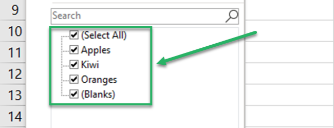
4. From these items, uncheck all others, except for ‘Apples’.

5. Click Okay, and you’re good to go!👍
6. Excel filters out the sales of ‘Apples’ only
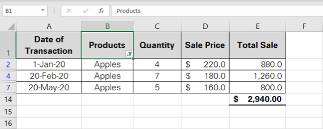
Quickly applying the SUM function to this sale tells that the total sales for Apples were $2940.
To save time that goes into checking and unchecking items, type the desired text (Apples) in the Search bar above and press Enter.
How to filter by numbers
Next is filtering in Excel using numbers.
The AutoFilter tool of Excel allows you to filter data based on numbers in a variety of ways.
Check out the variety of options in the image below.
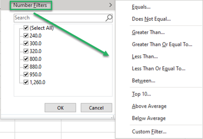
You can set up any parameter. Like filtering numbers that equal to say $1000 or are less / more than $1000 or whatever.
Alternatively, you can simply sort numbers in descending or ascending order.
In the above example, let’s apply a filter based on numbers. For instance, let’s filter out the sales that are equal to or less than $400.
1. Select the column for Total Sales and apply the filter tool to it.
2. Launch the filter tool by clicking on the drop-down arrow.
3. Go to Number Filters.
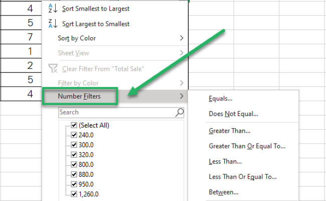
4. To filter out the sales that are equal to or less than $400, choose an appropriate parameter.
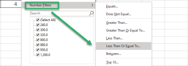
5. This launches the Custom AutoFilter dialog box.

6. Against the ‘Less than or Equal to’ tab, input the number ‘400.

7. Click Okay.
8. Excel filters the sales as follows.
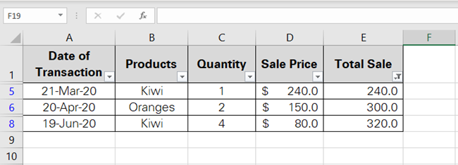
Excel has filtered out sales that were only equal to or less than $400.
Multiple filters simultaneously
Can you apply filters to multiple columns simultaneously?
For example, for the above data set, what if we want to filter out sales for Apples that are greater than $800?
This takes two filters:
- Text filters to filter out sales for the Product ‘Apples’.
- Number filters to filter out sales of Apples that exceed $800.
No worries. It’s still a piece of cake. See below.
1. Apply filters to the Product column.
2. From the filter drop-down menu, select ‘Apples’ to filter out sales for ‘Apples’ only.
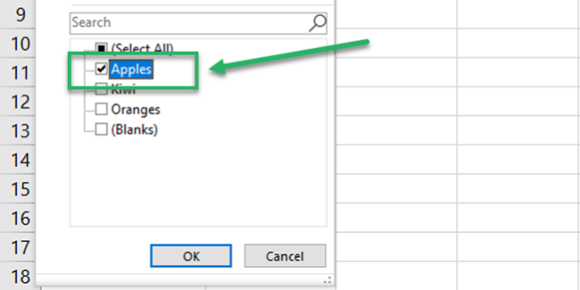
3. Click ‘Okay’ and Excel filters out the sales of ‘Apples’ only

4. Next, apply filters to the column ‘Total Sales.’
5. Launch the filter tool by clicking on the drop-down arrow against the column heading ‘Total Sales”.
6. Go to Number Filters.

7. To filter out the sales that are more than $800, choose an appropriate parameter.
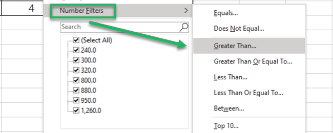
8. This launches the Custom AutoFilter dialog box. Against the ‘Greater than’ tab, input the number 800.

9. Click Okay, and Excel filters the sales as follows.

There you go! The AutoFilter tool filters out the sales of Apples that exceed $800.
You can apply as many filters as desired at any given time.
Pro Tip!
How do you know which columns of your data have the filter applied?🙋♂️
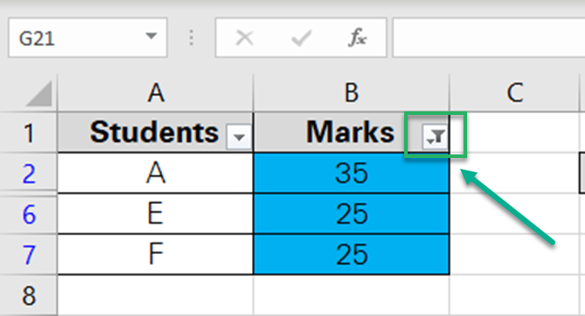
Look out for the filter (funnel) icon in place of the drop-down arrow. All the column headers that have this icon have the filter applied.
How to clear filters in Excel
There’s an undo to everything you do in Excel.
After you’ve applied filters to data, the drop-down menu for that column header takes a filter shape.
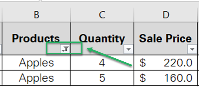
In this example, we have applied the filter to the column ‘Products’ to filter out the sales for ‘Apples’ only.
1. To remove this filter, go to the filter icon of the relevant column.
2. Launch the AutoFilter tool.
3. Select the option “Remove Filters.”
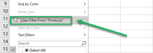
4. Alternatively, Go to Data > Sort & Filter > Clear.

5. This removes the filter “Apples” applied to Products.
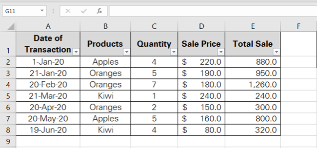
Excel now shows all the products (apples, oranges, and kiwi).
Also, note how the filter icon is now again replaced by the drop-down arrow.
How to remove filters entirely
In the above section, we’ve seen how to remove filters from a particular filter column.
But what if you want to remove filters from your data set entirely?
1. Select the data from where you want to remove filters.
2. Go to Data > Sort & Filter > Click Filter Button again.

This removes the AutoFilter from the data.
3. No more drop-down arrows.
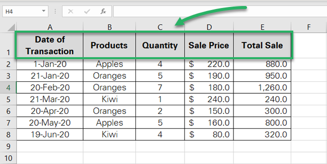
Remember the shortcut to Apply Filters? Control Key + Shift + L.
Press these three keys together to apply filters. Press them again together to remove the filters.
Filter by color in Excel
You can also use the AutoFilter Tool of Excel to filter out specific cells based on their color.
For example, the image below shows the marks of different students.
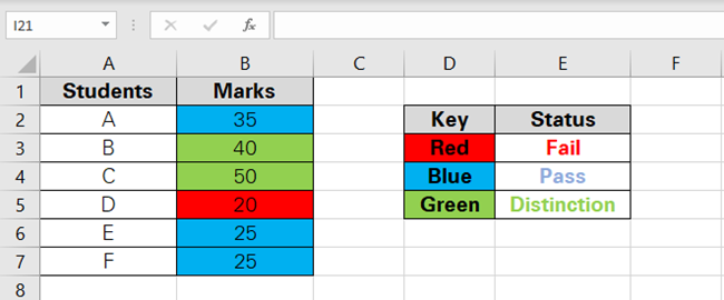
There’s also a key to the right side that tells how the coloring is done.
Let’s filter out the students who’ve passed.
1. Apply filters to the column that has the highlighted cells.
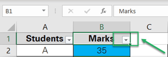
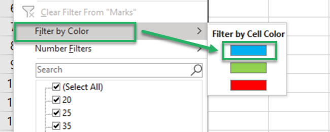
2. Launch the filter tool. Go to ‘Filter By Color’ and select the color blue.
We have selected the color blue as the key shows that the students who’ve passed are highlighted in blue.
And there you go! Excel only filters the cells that are highlighted in blue.
Advanced Filter in Excel
As the name suggests, advanced filters go a step beyond AutoFilters.
Using the advanced filters tool of Excel, you can apply multiple filters to your data at once.
1. Taking the data below for sales of different products as an example.
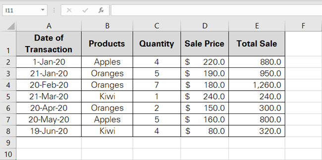
2. Let’s filter out sales for Oranges where the Quantity sold was 5 or more.
3. This involves two filters: Oranges and Qty of 5 or more.
4. To apply the Advanced filter, copy and paste the relevant headers of your data to separate cells. Relevant headers in this case are “Products” and “Quantity”

5. Under each header, mention the filter criteria as shown below.
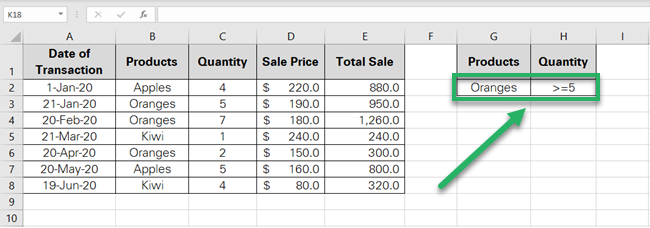
Under the Product header, we have mentioned ‘Oranges’.
Under the Quantity header, we have mentioned the criterion “>=5”
6. Go to Data > Sort & Filter > Advanced.

7. Against the List Range, select the data to be filtered.
8. Against the Criteria Range, select the formatted cells where the criterion is mentioned.
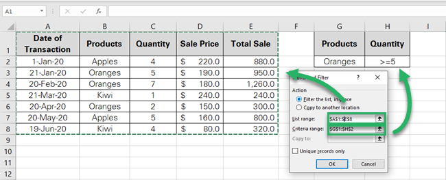
9. Hit Okay. Excel filters the data to show sales of Oranges of 5 or more units only.

Advanced filters allow you to apply many filters at the same time. It further allows you to filter data in its place or create a copy of filtered data to another destined place.
That’s it – Now what?
If you didn’t know about the filter tool of Excel yet, this guide is your savior.
We learned about filtering data based on text and numbers and colors in Excel using the Auto Filter tool. We also took a glance at the advanced filtering tool of Excel.
The filter and advanced filter tool of Excel will help you narrow down your data and pick out the relevant stats in an instant.
Especially, when used to assist other major functions like the VLOOKUP, SUMIF, and IF functions, it eases your Excel jobs by a thousand times.
Don’t know much about these functions? No worries.
Click here to sign up for my free 30-minute email course to help yourself learn these and many more amazing functions of Excel.
Other resources
If you enjoyed learning about AutoFilter and Advanced Filter in Excel, we bet you’d love to know more about the filter function and tools in Excel.
Check out our articles on data validation and creating data tables in Excel.
