How to Use the HLOOKUP Function in Excel: Step-by-Step
There are a total of four functions in Excel to look up a value. The LOOKUP, VLOOKUP, HLOOKUP, and XLOOKUP functions.
Each of these has a different purpose and is useful in its own way. The Excel HLOOKUP function looks up values in a table horizontally.
How? The following will guide and teach you that 👌
So continue reading and download our free sample workbook here to tag along with the guide.
Table of Contents
What is HLOOKUP in Excel?
HLOOKUP is a lookup function of Excel. H in HLOOKUP stands for horizontal – and the HLOOKUP function performs a horizontal lookup.
It looks for a given value in the first row of a table and returns the corresponding value from any row of that table (as specified).
For example, you can extract any data for the Companies (that are arranged horizontally) in this table by using the HLOOKUP function.
How about the number of employees for Company B? 📪
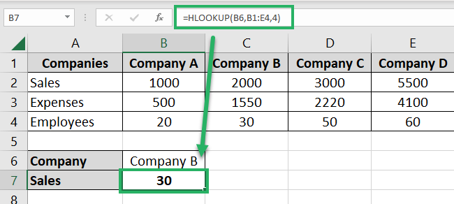
How to use HLOOKUP in Excel
Excited to see how the HLOOKUP function works in Excel? Here’s an example.
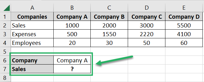
The image below represents some details for four companies.

We have the sales, the expenses and the number of employees for each company.
Did you note that the Companies are organized horizontally ❓
Now we want to find the Sales for any selected company instantly. Can we do that using the HLOOKUP function?
For example, for Company A?
Let’s see here.
- Write the HLOOKUP function as follows:
= HLOOKUP (
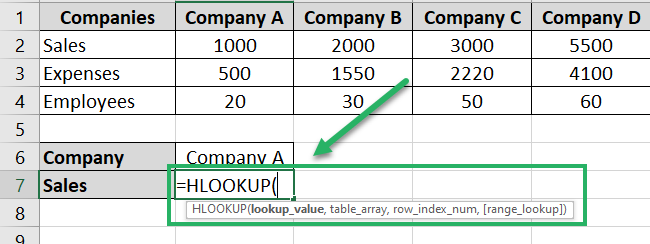
- Write the lookup_value as the first argument of the HLOOKUP function as below.
We want to find the sales for Company A. And as we have Company A written in a cell so, we will simply create a reference to it 🔁
= HLOOKUP (B6,
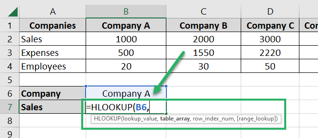
You can also input the text string “Company A” as the lookup_value yourself.
- As the table_array argument, refer to the table where HLOOKUP will look for the lookup_value.
The table in our case ranges from Cell B1 to E4.
= HLOOKUP (B6, B1:E4
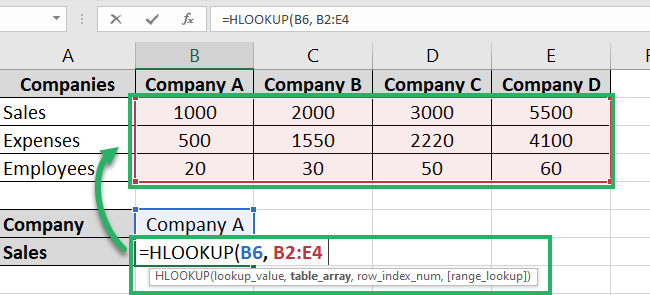
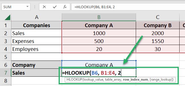
- As the row_index_num argument, specify the row number from where the matching value must be returned.
We want the sales for Company A to be returned. Sales sit in the second row in table B1:E4. So, we are setting the third argument to 2.
= HLOOKUP (B6, B1:E4, 2
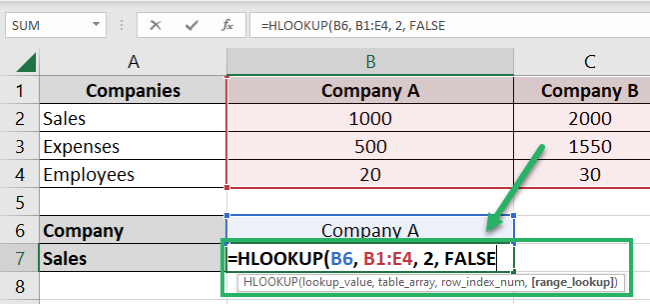
- As the range_lookup argument, write:
TRUE: If you want Excel to run an approximate match. In this case, the HLOOKUP will look up the exact value (Company A) or the next largest value less than this value.
FALSE: If you want Excel to run an exact match. In this case, the HLOOKUP will look up the exact value (Company A). And if the exact value is not found in the given table, it will return the #N/A error.
The range_lookup argument is an optional one. If omitted, Excel by default sets it to TRUE – approximate match mode 🎨
In this case, we are setting range_lookup to FALSE as we want HLOOKUP to perform an exact match.
= HLOOKUP (B6, B1:E4, 2, FALSE)
- Press Enter, and there you go.
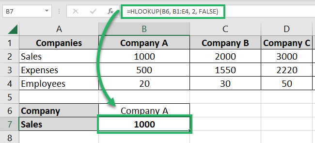
The HLOOKUP function fetches out the sales for Company A from the table above.
Simple enough 🙌
HLOOKUP formula example
Haven’t had enough of the HLOOKUP function yet? Same here 🤩
So let’s look into another (more interesting) example of the HLOOKUP function.
Here we have a list of participants for a marathon.

We can only choose a single participant from these. And the required height to choose one of them is 6 feet (or the nearest to it)🏃♂️
Now we don’t know if we have any participant who is exactly 6 feet tall. So we cannot run the HLOOKUP function with an exact lookup value of 6.
But we can go with an approximate match, no? So let’s do it.
Under the approximate match mode, the HLOOKUP function searches for the exact lookup value first 🎯
If the data doesn’t contain the exact lookup value, it then looks for the value that is the next largest but less than the lookup value itself.
- Begin writing the HLOOKUP function as follows:
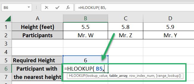
= HLOOKUP ( B5
Alt-text: Lookup_value of the HLOOKUP function
We have created a reference to Cell B5 as it contains our lookup value i.e. 6.
- As the second argument, specify the table where the value must be looked up.
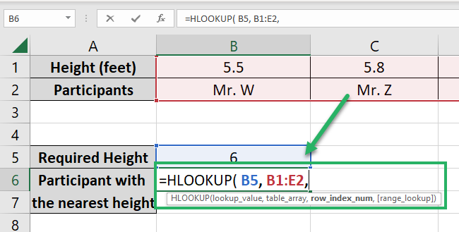
For our example, it ranges from Cell B1 to E2.
= HLOOKUP ( B5, B1:E2
- Next, specify the row from where the corresponding value must be returned.
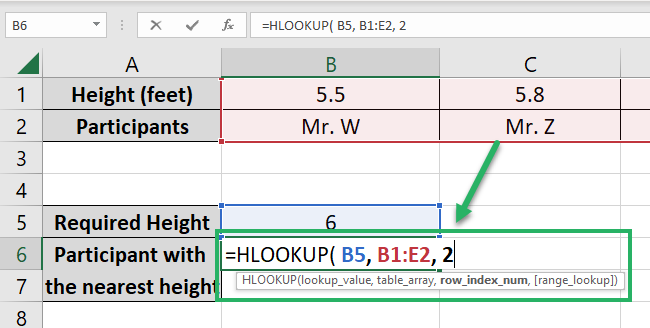
We need the name of the participant (that sits in row 1 of table B1:E2). And so, we are selecting 2 as the row_index_num argument.
= HLOOKUP (B5, B1:E2, 2
- Set the range_lookup to TRUE.
= HLOOKUP ( B5, B1:E2, 2, “TRUE”)
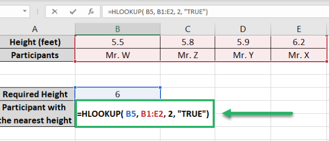
We have set the range_lookup to TRUE, which is an approximate match mode. This is because we are not yet sure if the list above has any participant who is exactly 6 feet tall.
So we want to pick out any participant who is 6 feet tall. And if there is no such participant, then the one who is nearest to 6 feet tall.
Pro Tip!
To run an approximate match under the HLOOKUP function, the values in the first row of your table must be sorted in ascending order 🔠
The first row is where the HLOOKUP function looks for the lookup_value. Unless it is arranged in ascending order, the HLOOKUP function might not return the correct results.
Note that the heights in our dataset above are arranged in ascending order. Starting from 5.5 inches (the leftmost value) up to 6.2 inches (the rightmost value).
- Hit “Enter” to get the results as follows:
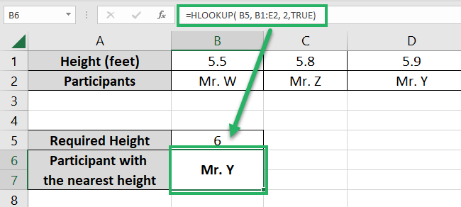
And the HLOOKUP function has nominated Mr. Y as the marathon participant 💪
But did you note? The height of Mr. Y is not 6 feet but only 5.9 feet.
However, as none of the participants from the list have a 6 feet height, the approximate mode of HLOOKUP activates 📍
And it looks for the value next largest but less than the lookup value of 6. The next smallest value is 5.9 feet, and so the result is Mr. Y.
That’s it – Now what?
That was all about the Microsoft Excel HLOOKUP function. Through the guide above, we have looked into each argument of the HLOOKUP function.
We have also seen multiple examples of how the HLOOKUP function might be used in Excel. The lookup functions of Excel are a blessing – and the HLOOKUP function is no different.
If you enjoyed learning about the HLOOKUP function, you’d love to know about other functions of Excel too.
Like the VLOOKUP (the twin of the HLOOKUP function), SUMIF, and IF functions of Excel.
Other resources
The HLOOKUP function of Excel helps the horizontal lookup of values. But if you have your data organized as columns and not as rows, the HLOOKUP function might not help you enough.
👉 To search such data types, you need the VLOOKUP function – learn how to use it by clicking here.
In addition to the VLOOKUP function, the modern XLOOKUP function helps search data both ways – vertically and horizontally. Learn it here.
