How to Use XLOOKUP in Excel: Step-By-Step + Examples (2024)

If you’ve heard great things about XLOOKUP – you heard right!

Excel’s new XLOOKUP function is an improvement over the old (but very popular) VLOOKUP function.

Compared to other lookup functions, XLOOKUP:

• Has built-in error handling
• Can return multiple results (!)
• Is much easier to use

If you master the XLOOKUP function, you can easily replace VLOOKUP, HLOOKUP, and maybe even INDEX MATCH🔍

Click here to download the Excel spreadsheet and tag along.

How to use XLOOKUP (the simple way)

Basically, you have to give only 3 parameters for XLOOKUP in excel.

• Lookup value – The value that you need to search.
• Lookup array – The search array for the lookup value.
• Return array – The array to consider for the result.

Sounds easy, right? 😎

We will start the XLOOKUP function with a simple example.

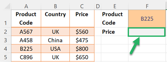
Let’s use the XLOOKUP function and find the price for the given product code in cell F1.

1. Enter an equal sign and start the XLOOKUP function.

=XLOOKUP(

2. Make a reference to the lookup value.

In this case, the lookup value is the product code we are looking for.

The XLOOKUP formula now looks like this:

=XLOOKUP(F1

3. Select the lookup array. This is the column to look for a match with the lookup value.

In this case, look for the product code (lookup value) in the column with product codes (column A).

=XLOOKUP(F1,A2:A7

4. Select the return array to get the result.

Because we want to return the price, select the price column.

Now, your XLOOKUP function looks like this;

=XLOOKUP(F1,A2:A7,C2:C7

5. Close the parenthesis and press Enter.

The XLOOKUP function in the F2 cell should be;

=XLOOKUP(F1,A2:A7,C2:C7)

XLOOKUP will find the exact match of the product code in column A and return the price (from column C) in the same row.

This is the basic functionality of any lookup function/formula. But the way you just did it with XLOOKUP is much easier than with VLOOKUP or INDEX MATCH.

The new XLOOKUP has 3 other optional parameters.

Let’s explore the advanced options of XLOOKUP 🤔

Advanced options of XLOOKUP

Not found message

#N/A error is a very common error in lookup functions.

It happens when the lookup value does not exist in the lookup table.

The solution for the #N/A error was to use IFERROR or IFNA.

This is no longer necessary with XLOOKUP.

You just need to use the optional fourth argument of XLOOKUP [If not found].

If the value does not exist in the lookup array, indicate the value to be returned.

Let’s modify the XLOOKUP formula of the above example as follows.

=XLOOKUP(F1,A2:A7,C2:C7,”Check the code”)

Now change the product code to a code that is not in the data set.

If no valid match is found and [if not found] is not given, XLOOKUP returns the #N/A error.

Pro Tip!

The XLOOKUP can only do one lookup per data set.

Do you want to do a lookup across multiple sets of data that are saved in different sheets?

You can nest another XLOOKUP in the fourth argument (i.e., if not found) of the XLOOKUP Function.

Match type

The XLOOKUP function can return results for exact matches as well as for approximate matches.

This is the fifth argument of the XLOOKUP.la.

If you do not specify the match mode, the default value of 0 will be considered.

As a result, the function will return only the exact match.

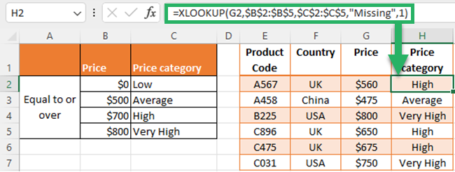
-1 and 1 are very useful when you have thresholds.

-1 will return the exact match or the next smaller matching value.

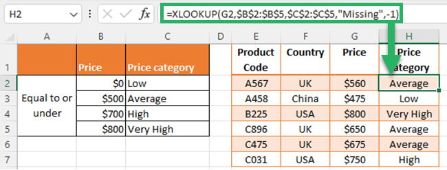
1 will return the exact match or the next larger matching value.

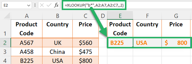
To get a partial match lookup value, enter 2 for the match mode.

Then, you can do a wildcard character match.

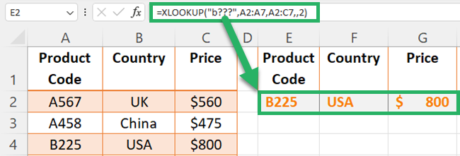
The below 2 example shows the XLOOKUP formula where the lookup value is given with wildcard match mode.

Let’s match product codes that start with the letter “B”.

Search mode

Unlike the VLOOKUP function, the XLOOKUP function in Excel has 4 search mode options 😯

We can search a lookup value starting from the first value or the last matching value.

You can even perform a binary search for the lookup value.

The below example spreadsheet shows the XLOOKUP function with search lookup value first-to-last.

We want to get product codes starting with the letter “A”.

The below image shows the same example with the search mode -1 which is the search lookup value last-to-first value.

You can enter 2 for search mode and do a binary search from the first-to-last matching value if you have sorted the lookup array in ascending order.

You can enter -2 for search mode and do a binary search from the last-to-first matching value if you have sorted the lookup array in descending order.

More XLOOKUP formula examples

Now, it’s time to learn the wonders of the XLOOKUP formula using the below XLOOKUP examples.

XLOOKUP formula example #1

We can use nested XLOOKUP functions to combine vertical lookup and horizontal lookup.

In the below example, we need to find the net profit for March.

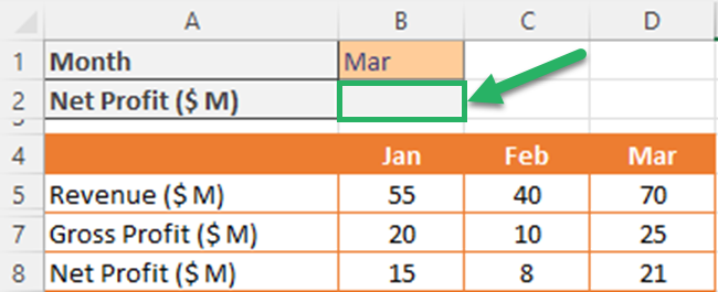
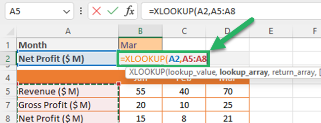
1. Search “Net Profit ($ M)” from “column A” using the XLOOKUP function.

Now the formula is;

=XLOOKUP(A2,A5:A8

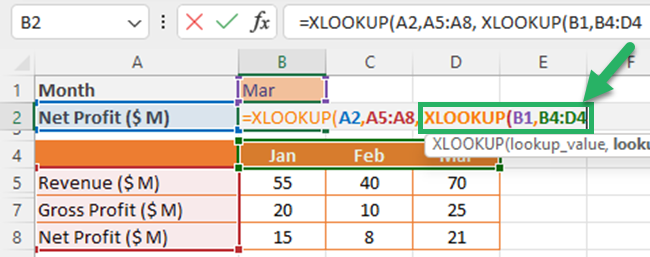
2. Finding the month as a horizontal lookup value by the Excel XLOOKUP function.

After entering the new function, the formula is;

=XLOOKUP(A2,A5:A8,XLOOKUP(B1,B4:D4

3. Enter the XLOOKUP return array in the outer XLOOKUP formula.

Give cell references to all the values in the data set.

Now your formula is;

=XLOOKUP(A2,A5:A8,XLOOKUP(B1,B4:D4,B5:D8

4. Close all the parentheses and press the “Enter” key.

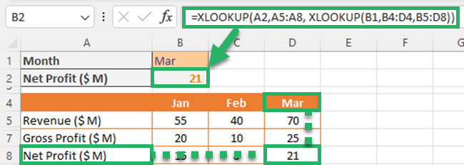
The above formula works as a two-way lookup and returns the value at the intersection of the two.

Isn’t it easier than the traditional INDEX MATCH method? 🥳

XLOOKUP formula example #2

You can also use nested XLOOKUP functions in Excel with the SUM function and get the total between two ranges.

Let’s use the below example in the Excel file.

1. First, enter the SUM function in excel.

The Formula is;

=SUM(

2. Enter an XLOOKUP and search the net profit of the start month.

=SUM(XLOOKUP(B2,B4:D4,B5:D5)

3. Enter a colon symbol to get the net profit of the end month using the XLOOKUP formula.

The updated formula is;

=SUM(XLOOKUP(B2,B4:D4,B5:D5):XLOOKUP(C2,B4:D4,B5:D5)

4. Close the parenthesis and press the “Enter” key.

You can get the total net profit between February to March.

The above formula can be used to get the total of a dynamic array.

That’s it – Now what?

Now you are proficient with the XLOOKUP – superhero of the lookup functions 🥳

You can easily replace many complicated functions with XLOOKUP.

You can also combine XLOOKUP with SUM, COUNT, and AVERAGE functions and get more dynamic results for your financial models.

But XLOOKUP is not the only important function out there at all 🙋🏻‍♂️

Functions like IF and SUMIF are other ‘Hall of Famers that you absolutely need to learn.

Click here to enroll in my free 30-minute online course and learn IF, SUMIF, and data cleaning.

Other resources

The XLOOKUP function is currently available to Microsoft 365 Excel users.

You can read our article about Microsoft 365 to understand its best features 😍

If you don’t have Microsoft 365 there are other great lookup options like VLOOKUP, HLOOKUP, and INDEX MATCH.

Frequently asked questions