How to Use the IFNA Function in Excel: Step-by-Step
Are you done with the #N/A errors all spread over your Excel sheet? Want to get rid of them?
The IFNA function is all that you need 🏃♀️
With the IFNA function, you can replace the #N/A error in Excel with any custom text.
Want to see how this works? Slide straight into the guide below and download our free sample workbook here to tag along with the guide.
Table of Contents
What to use IFNA for?
The #N/A error is Excel’s way of saying that the value you’ve been looking for is not there in the lookup array or table.
The IFNA function is meant to help you identify, track and handle the #N/A errors in Excel 🔎
It evaluates if a given formula results in the #N/A error. If it does, the IFNA function will replace the #N/A error with any text you like. And if it doesn’t, the IFNA function will simply return the formula results.
So you can use this function to steer your spreadsheet clear of the unpleasant #N/A errors 🧹
How to use IFNA
Let us now see how you can use the IFNA function in Excel. So here’s a dataset that contains the roll numbers, names, and marks of different students.
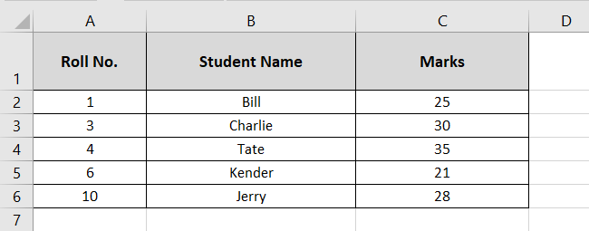
And here we have another table where we want to fetch the marks of each roll number.
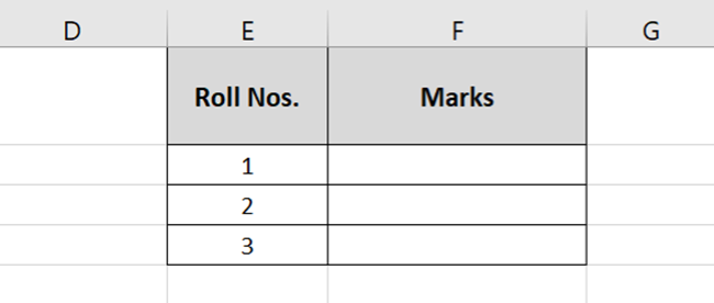
Note that the table where we want the marks contains some roll numbers that are not present in the first table (Roll No. 2) 🙈
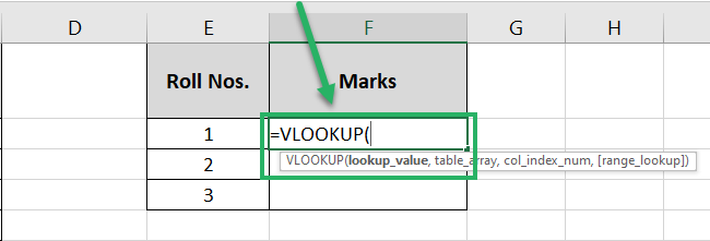
Let’s write the VLOOKUP function to find the marks for each roll number from the first table.
- Begin writing the VLOOKUP function as follows.
= VLOOKUP (
- Define the lookup value. We are setting it to Cell E2 as it contains the roll number.
= VLOOKUP (E2,

- Refer to the lookup range (where the lookup value is to be looked for). This is the table that contains all the data i.e. $A$2:$C$6.
= VLOOKUP (E2, $A$2:$C$6

It is important to change the lookup range reference to an absolute reference. This is to ensure the lookup range reference remains unchanged when we drag and drop the formula 📜
- Define the column index number from where the value must be returned. We need the marks for the given roll number.
Marks sit in Column 3 of the lookup range so we are defining the col_index_num as 3.
= VLOOKUP (E2, $A$2:$C$6, 3
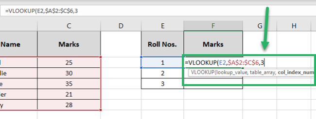
- Set the match mode to ‘Exact Match’ by setting the last argument to FALSE.
= VLOOKUP (E2, $A$2:$C$6, 3, FALSE)
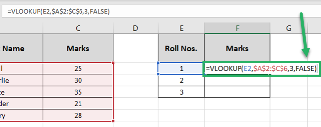
With this, Excel will look for the exact roll number only 💡
Pro Tip!
The match mode is an optional argument.
If omitted, Excel sets it to TRUE (Approximate Match Mode), by default.
Under the approximate match mode, Excel looks for the lookup value or the next smallest value (if the lookup value doesn’t exist in the lookup range).
Whereas the under the EXACT match mode (FALSE), Excel looks for the lookup value. If the lookup value is not available, it returns the #N/A error ❌
- Hit Enter, and here come the results. We get the marks for Roll Number 1 that are 25.
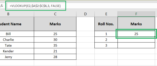
- Drag and drop the same to the remaining roll numbers. And this is what happens.
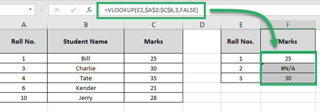
For Roll Number 2, we get the #N/A error. This is because Roll No. 2 doesn’t exist in the first table. So Excel tells you ‘Not available through the #N/A error 🚩
And all of a sudden, the table starts to look all the odder because of the #N/A error in between. Want to get rid of it?
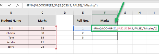
8. For that, nest the formula above in the IFNA function as follows:
IFNA (VLOOKUP (E2, $A$2:$C$6, 3, FALSE), “Missing”)
Pro Tip!
The first argument of the IFNA function is the value (or the function) to be evaluated for the #N/A error. We have replaced it with the VLOOKUP function above 👆
And the second argument is the value_if_na. We have set it to “Missing” (do not miss out on the double quotation marks).
This tells Excel to check if the given formula returns the #N/A error. If it does, the IFNA function will replace it with the value supplied as the value_if_na argument.
If it doesn’t, the result of the formula will be returned. The IFNA function works like a logical function ✌
- Hit Enter.
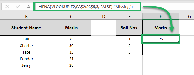
The result is still 25.
- Drag and drop the formula to the whole list.
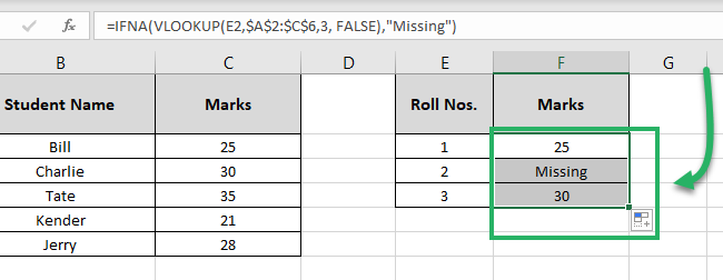
IFNA turns the result for Roll No. 2 to “Missing” whereas, for the other two roll numbers, it returns their marks.
This is because Roll No. 2 is missing in the first table. When the lookup value is missing from the lookup range, the VLOOKUP function returns the #N/A error.
And the IFNA function replaces the #N/A error with the supplied text i.e. “Missing”.
For the other roll numbers (that are present in the first table), the VLOOKUP function returns the corresponding marks 🎓
That’s how you can use the IFNA function to handle and replace the #N/A errors in your spreadsheet. Fun, no?
IFNA vs. IFERROR
The IFERROR function works the same as the IFNA function.
However, the only difference is that the IFNA function only identifies and replaces the #N/A error. Whereas the IFERROR function identifies and replaces all kinds of errors that Excel may pose 🧐
For example, let’s nest the above VLOOKUP function in the IFERROR function.
= IFERROR (VLOOKUP (E2, $A$2:$C$6, 3, FALSE), “Missing”)
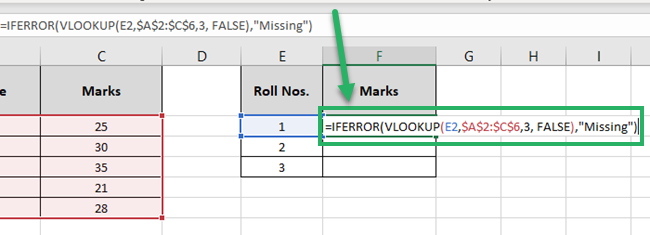
The results will still be the same.
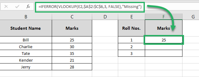
That’s because the IFERROR function can evaluate all kinds of errors and replace them with the specified text.
So, even if we rewrite the above function as follows:
= VLOOUP (E2, $A$2:$C$6, 3, FALSE)
We have misspelled the VLOOKUP function as VLOOUP. In such a case, Excel returns the #NAME? Error. See for yourself 👀
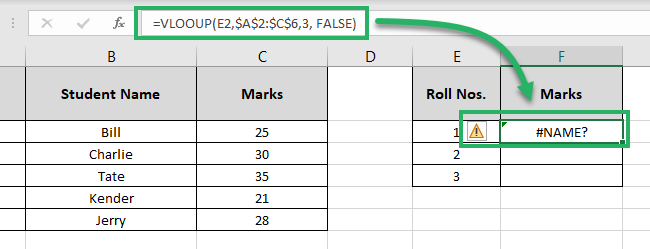
Now nest it in the IFERROR function as below.
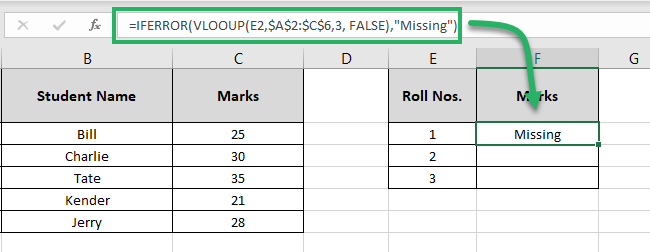
= IFERROR (VLOOUP (E2, $A$2:$C$6, 3, FALSE), “Missing”)
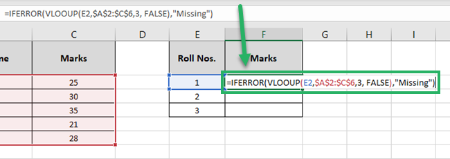
The IFERROR function will replace the #NAME error with the supplied value argument i.e. “Missing” too.
However, if we nest the same formula in the IFNA function, the results would have been different.
= IFNA (VLOOUP (E2, $A$2:$C$6, 3, FALSE), “Missing”)
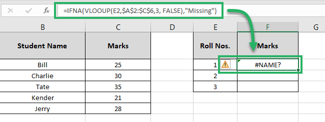
We still get the #NAME error. That’s because the IFNA function can only handle the #N/A error and no other errors 🤷♀️
Pro Tip!
The IFERROR function is a versatile Excel function that will save you against all Excel errors.
But if you are only targeting the #N/A error, it’s always better to go with the IFNA function instead. This will help you identify if the subject error was a #N/A error or any other ✍
That’s it – Now what?
That’s all about the super useful Excel IFNA function. It helps you evaluate formulas for the #N/A error and replace them (if any) with any text of your choice.
Isn’t that just so cool? MS Excel offers many more tools, features, and functions that’ll leave you equally amazed. The collection is huge.
To start with, I suggest you go with the VLOOKUP, SUMIF, and IF functions. These are some of the easiest yet most useful functions of Excel 🔔
Other resources
Want to learn more about the IFERROR function? Read our blog on it.
It will help you handle and replace all kinds of Excel errors. A true lifesaver!
