How to Use the IFERROR Function in Excel (+ ISERROR)
The IFERROR function checks if a formula returns an error.
If it does, the IFERROR function forces something to happen, like displaying an error message or value specified by you. Or running another formula.
This makes it insanely valuable to trap and handle errors in Excel formulas.
The ISERROR function is similar, but at the same time very different.
I’ll walk you through how to use both step-by-step in the following guide 🚀
Oh, and click here to download our sample workbook to tag along.
Table of Contents
How to use IFERROR
The IFERROR function has two arguments:
=IFERROR (value, value_if_error)
- ‘value‘- This is the expression (formula) that the IFERROR function tests for any error.
- ‘value_if_error‘- This is the value supplied by us. The IFERROR function returns this value if it finds the subject formula erroneous.
Pro Tip!
The IFERROR function tests the following errors:
- #N/A
- #VALUE!
- #REF!
- #DIV/0!
- #NUM!
- #NAME?
- #NULL!
To see the IFERROR function in action, check out the data below 🙌
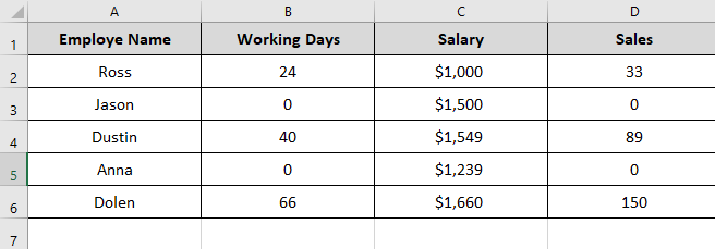
The data above represents the working days of employees, their salaries, and the sales won by them.
How can you calculate the sales efficiency of each employee from the data above?
By simply dividing each employee’s sales (Column D) by his working days (Column B).
=D2/B2
Drag and drop the same formula to the whole list.
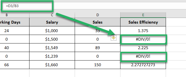
But what is that? Why is there a #DIV/0 error message in cells E3 and E5? This is because the dividend i.e. Working Days for cells E3 and E5 are zero.
Let’s rerun the formula above, but this time with the IFERROR function.
=IFERROR(D3/B3 , 0)
Enclose the above formula in the IFERROR function. And in place of the value_if_error argument, specify zero (o).
Here is what the results now look like:
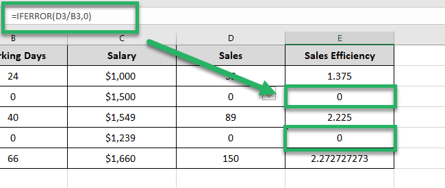
This time, instead of displaying an error message (#DIV/0!), excel returned zero for Cell E3 and E5.
Here’s what happened above:
- The IFERROR function checked the formula (Sales/Working Days) for any error.
- It found two #DIV/0! errors in Cell E3 and E5.
- For each of these cells, the error dialogue (#DIV/0!) was replaced by 0 (the value_if_error specified by us).
Easy enough💯
Using the IFERROR function, you can display any custom message in place of an error dialogue.
For example, you may rewrite the IFERROR function above as follows:
=IFERROR(D3/B3,”On Leave”)
This time the value_if_error is “On Leave” and so, the results change as follows:
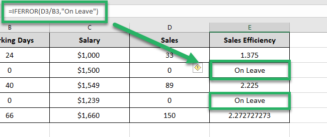
This means we can now finally say goodbye to the not-so-pleasant error messages posed by Excel.
A Yay moment 🤩
IFERROR VLOOKUP formula example
With the VLOOKUP function, we often face situations where the value we are looking for does not exist in the lookup table. In such cases, Excel returns the ‘#N/A’ error.
And we know how disturbing this looks 🙄 But we can now fix these error messages.
How? Take a look at the data below.
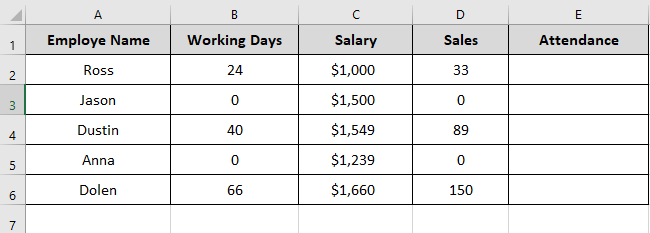
The above image consists of details of different employees of a company.
Let’s see which of these employees attended office by matching the attendance column above with the lookup table below.
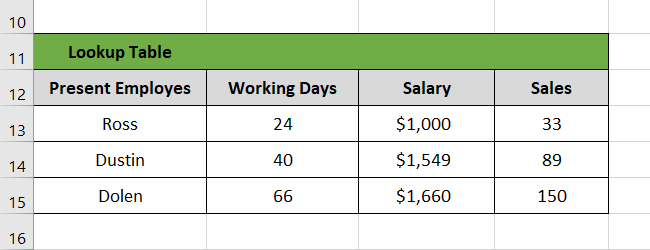
To do so, write the VLOOKUP formula as follows:
=VLOOKUP(A3,A13:A15,1,0)

The list of present employees did not contain the names “Jason and Anna”.
And so, the VLOOKUP function returns an ‘#N/A’ error for both of them.
But hold on 🤚 We don’t want the very annoying #N/A error on our sheet. Instead, we want a simple “Absent” status for the employees not present in the lookup table.
To do this, we must nest the VLOOKUP function above in the IFERROR function:
= IFERROR (VLOOKUP (A5,A13:A15,1,0),”Absent”)
Note that we have specified the value_if_error as “Absent”.
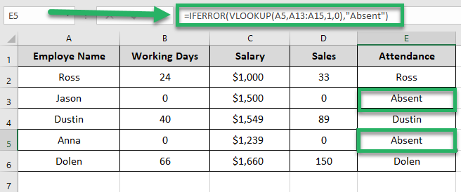
See the change 👀
Instead of the #N/A error, Excel returned the value “Absent” for the employees missing from the lookup table.
How to use ISERROR
Now comes the ISERROR function.
Unlike the IFERROR function, the ISERROR function only tells if there is or isn’t an error in the formula. And so, it’s way simpler to use.
Ready to see it into action? Take a look at the image below.
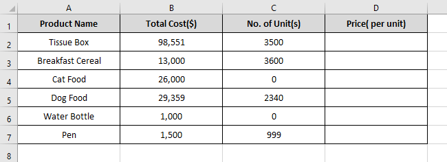
The data above represents the cost and units of different items bought by a local grocery store.
While we know the total cost for each item above, we don’t know their cost per unit.
To find it, simply divide the total cost of each item (Column B) by the number of units bought (Column C).
= B2/C2
And here’s what you get out of it.
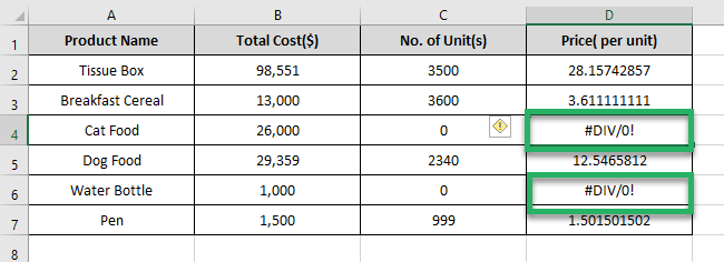
While we easily calculated the cost per unit for all the other items, for cells D4 and D6, we only have a ‘#DIV/0!’ error.
Is there some way to identify such errors before we apply any formula 🚩
To know beforehand if your formula is an erroneous one or not, use the ISERROR function as follows:
=ISERROR(B2/C2)
Drag and drop the above formula to the whole list to find a Boolean result (True/False) for each item.
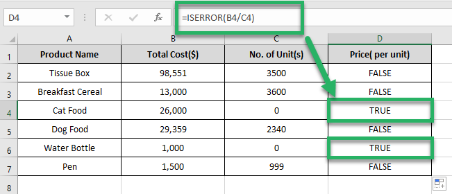
The Excel ISERROR function tests the same set of errors as the IFERROR function does.
For two items, the Cat Food and Water Bottle, the ISERROR function returns a True value. These are the same two items for which we had a #DIV/0! error earlier.
What does this mean? The ISERROR function tests a formula to be erroneous or not.
If it results in an error (like the #DIV/0 error above), the function returns “True”. And if the result of the formula is not an error, the ISERROR function returns “False”.
Pro Tip!💡
You may use an array formula (like B2:B7/C2:C7) to check a long list of formulas. This saves you time and prevents unwanted errors by checking all the formulas in one go 💡
IF ISERROR formula example
The ISERROR function simply checks a formula for any error and returns True/False as the result. It doesn’t allow users to specify a particular value to be returned in place of True/False.
As the ISERROR doesn’t allow for this by default, you can still do so by nesting it in the IF function.
The IF function performs a logical test and works the same way as the IFERROR function.
- Write the IF function as follows:
=IF(ISERROR(B2:B8/C2:C8),”On Route”, B2:B8/C2:C8)
Pro Tip!
Here’s how both these functions work:
- The first argument is a logical test. We have nested the ISERROR in its place which will perform a logical test on the value and return True/False.
- The second argument specifies the value (“On Route”) to be returned by the IF function if the logical test turns out true.
- The third argument specifies the value (the result of the division function) to be returned by the IF function if the logical test turns about false.
- Press down the Control key + Shift key + Enter.
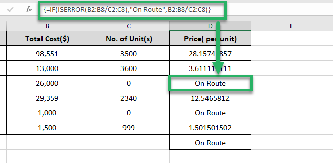
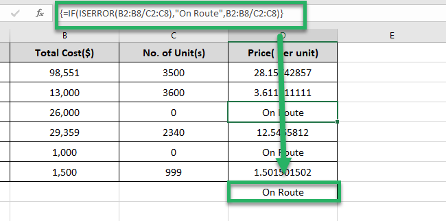
The formula above is an array formula – note that the formula is enclosed in curly brackets 😵
An array formula is a formula whose result extends to an array of cells and not a single cell. To complete array formulas, you don’t simply hit Enter but Control + Shift + Enter.
See how the two functions worked together to give us our desired results.
For cells where the formula doesn’t result in an error – we have the cost per unit calculated for the relevant item. And for the cells where the formula returns an error, Excel returned the value “On Route”.
Note that in the above example, the selected range also includes a blank cell (Cell D8). As both the relevant cells (Cell B8 and C8) were blank, cell D8 must return a #DIV/0 error.
And the IF function together with the ISERROR function returned the value “On Route” for Cell D8.
Pro Tip!
The IFERROR function performs almost the same job as the ISERROR function combined with the IF function.
The only difference is that the IFERROR function doesn’t let you specify the value_if_false argument ❌
IFERROR vs ISERROR
Both the IFERROR and the ISERROR functions are used to identify an error. But they are still different in the following aspects:
- The ISERROR function only tells if the subject formula returns an error or not.
- It only returns Boolean values (True/False) as results.
- On the other hand, the IFERROR function checks a formula for any error.
- It further allows users to define a value to replace the error (if there exists any).
All in all, the IFERROR function is a more dynamic and user-friendly function than ISERROR✔
But both these functions can become all the more beneficial when used together with other functions. Like the SUM function, or the VLOOKUP function.
That’s it – Now what?
That’s all about using the IFERROR and ISERROR functions in Excel.
In the guide above, we have not only seen how to use both these functions but also how they might be nested into other functions for better results.
While these are some of the fundamental functions of Excel, do know that the Excel function library has much more than this to offer.
Some principal functions of Excel include the VLOOKUP, IF, and SUMIF functions💪
Want to master them? Register for my 30-minute free email course to get your hands on these (and many more) functions of Excel.
Other resources
The IF and IFS functions are some of the most versatile functions of Excel. However, when used together with other functions, they might pose some unexpected errors.
To learn more about the errors posed by the IFS function, click here.
Or if you’re wondering why these errors even pop up in the first place? Learn and fix this here.
