How to Name Columns in Excel (The Easiest Method)
An Excel spreadsheet is a two-dimensional set of cells. The grid of cells that runs horizontally is called a row.
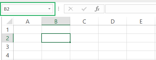
And the cells that run vertically make a column. By default, Excel columns are named based on alphabets starting from A up to XFD which makes 16,384 columns. Wow-worthy number 🤩
In any case, if you do not like how these columns are named in Excel, you are not bound to go with the alphabetical names. You can name them as you like.
In this tutorial, we will see quite a few methods to name columns in Excel. To learn these methods with us, download the free practice workbook for this guide here and stay tuned till the end.
Type in the Column Header in the first row
The first method is to add a column header for your data (after the Excel column headers) to name columns in Excel.
For example, I have a list of data populated in Excel 📝
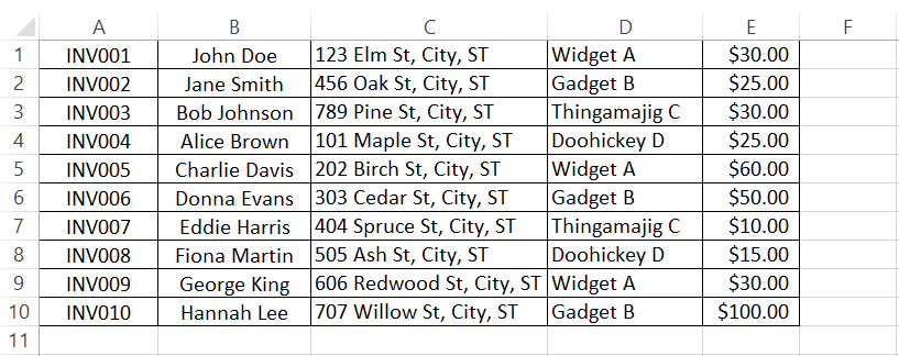
To name these columns:
Step 1) Go to the first cell of any column.
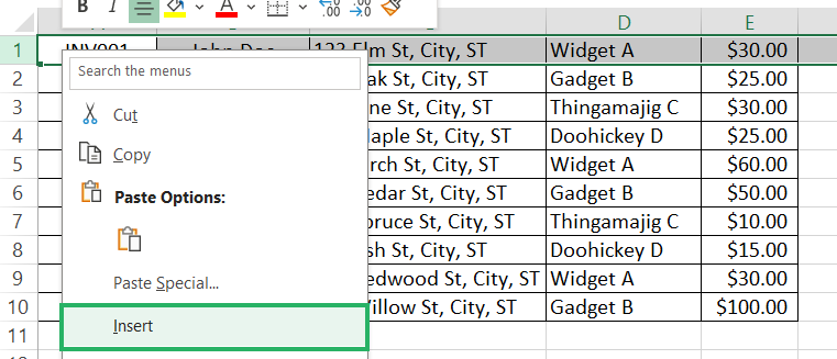
Step 2) Right-click to launch the context menu.
Step 3) Click on the Insert.
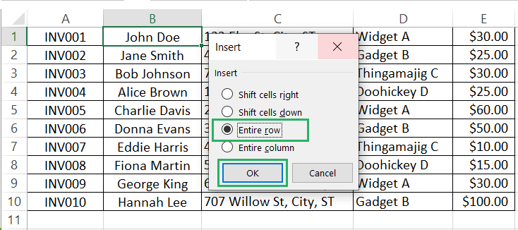
Step 4) From the insert menu, select Entire row and click Enter.
You can insert a new row by pressing the keyboard shortcut key of Shift key + Control key + Plus sign (+).
A new row will be inserted above your data.
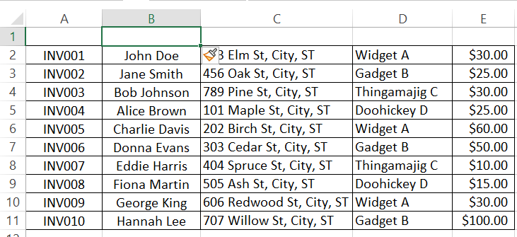
Step 5) In this row, type the column header names as you desire.

You can then format them to be bold or however, you like to give them name-like prominence.

These column headers will help you identify the columns by the names you want. But Excel still knows them by their alphabetical names 🔡
If you want Excel to know them by these names (that we just entered), follow the next section.
Name Columns in Excel from Selection
Once you have named the columns in your data by writing a column header, you can tell Excel to save these headings as the column names by following these steps 👇
Step 1) Select the columns that you want to be named based on their headers.
Step 2) Go to the Formulas tab > Defined Names > Create from selection.

Step 3) Select the option to create column names from Top Rows.
Step 4) Press okay.
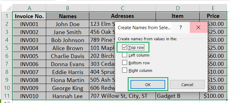
From the column headings in the Top Row, Excel has created column names.
Now when you type this name in any cell in a formula or simply after an equal sign, Excel will identify it as the name of that relevant column.

We had selected only the cells containing the data, so the column name Item only includes Cell D2 to D11.
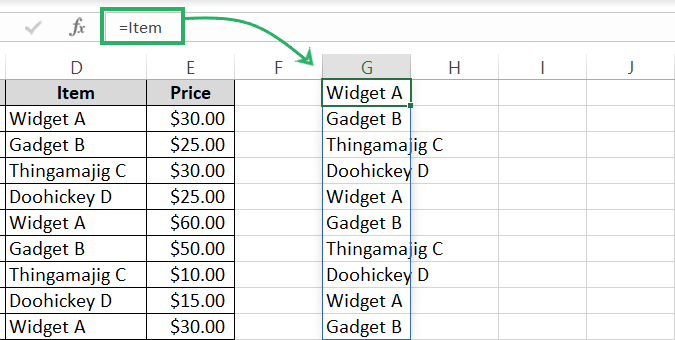
Under each column name, only those cells that you selected while converting the header into column name. If you selected the entire columns, then the name would cover the entire column. If you selected only certain cells, say A2:A10, only these will be covered by the column name for Column A.
Name Columns in Excel from the Name Box
Another way to name columns is to name them from the Name box 🎯
Step 1) Select the column that you want to name by clicking on the column header as highlighted below.
This will automatically select the whole column.

Step 2) Go to the Name box.
Step 3) Type the name that you want for this column.

Step 4) Press Enter.
Excel will save this column by the name given by you.
Check this out:

This is the easiest method to name columns in Excel.
Name Column in Excel from Name Manager
The Name Manager in Excel stores the names for all the named items in Excel. These can be cell names, named ranges, table names, or anything else 😲
To name a column:
Step 1) Select the column to be named from by clicking on its header.
Step 2) Go to the Formulas tab > Define names > Name manager.

The Name Manager dialog box will launch before you.
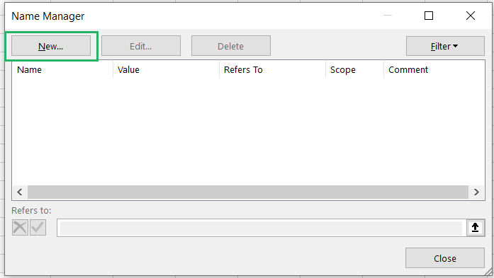
Step 3) Click on the New button.
Step 4) Within the New Name box, write the name you want for the column.
Step 5) Set the scope of this name to extend across the active sheet only or the whole workbook (in which case you’d be able to refer to this column with its name in any sheet of the workbook).
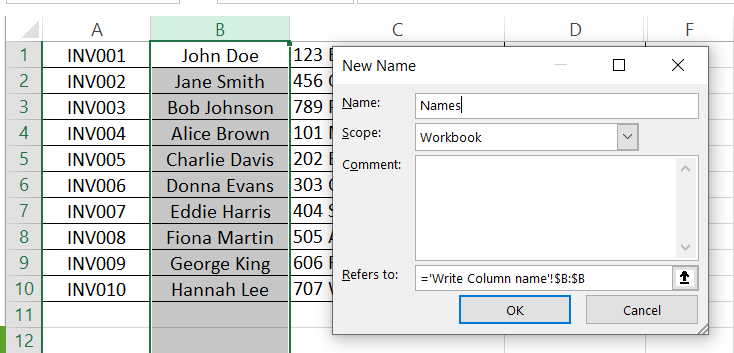
Step 6) Click on okay to save the name.
Now when you again launch the Name Manager from the Formulas tab > Define Name > Name Manager, you’ll see the name saved there 🚀
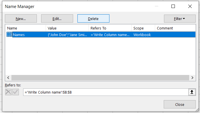
Excel now knows this column by the designated name, and you can refer to it anywhere around the sheet or workbook (depending upon the scope you’ve set).

You can use it in formulas and use it as a reference just like you use any normal cell reference.

The Name Manager gives you a quick view of all the names defined in Excel.
Name Columns in Excel in R1C1 Style
This is not really about naming columns to your choice.
But if you’re bored of looking at the same alphabetically designated columns or for any other reason, you do not want the columns to be named by A, B, or C but, as 1,2,3, you can opt for the R1C1 reference style 🔢
Here’s how you can apply it in Excel.
Step 1) Go to the File tab > Options.
Step 2) Go to Formulas from the pane on the left.
Step 3) Under the head Working with Formulas, check the option for R1C1 reference style.
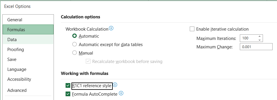
Step 4) Click okay.
Come back to your sheet to see all the column headers are changed from column letters to numbers. The cell reference in the name box is now in the R1C1 style 💡
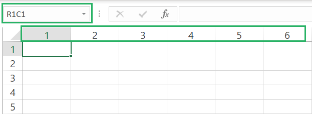
If you ecide to change this style anytime later, go back to the Excel options and uncheck the R1C1 reference style.
The column headers will get back to alphabetic denotation.
Conclusion
This guide entails a whole list of stellar methods to change the column names in your Excel sheet each of which is explained step-by-step.
Naming columns in Microsoft Excel can help you with referencing them later around your sheet or workbook. And sometimes, maybe it’s just about how you want your sheet to look 👀
In addition to naming columns, here are some other Excel tutorials that discuss how you can name sheets and ranges in Excel.
