How to Calculate NPV Using Excel
(NPV Formula Explained)
Net present value is a core topic of Financial Modeling.
It discounts future cash flows to show their today’s value 📆
But you’re not a finance person? That’s alright. In the tutorial below, I am going to explain to you the concept of NPV, multiple ways to calculate NPV in Excel, and the different functions that Excel offers for NPV calculation.
So, grab your practice workbook for this tutorial here since it’s going to get more and more interesting with every next section. And let’s dive in straight.
What is NPV?
Net present value means the net value of an investment today. It is a financial measure to tell if an investment is going to be profitable or if it is worth investing in.
To calculate NPV, we estimate the cashflows (outflows and inflows) to be generated from a project. So, let’s say I plan on establishing a car rental business 🚚
To decide if it is financially feasible to invest in it, I will see what investment it takes. Let’s say it takes me 3 cars worth $2000 each to set up the business initially.
Cool – next, I will see what return I expect to generate from it. Say $2500 for the next 5 years each.
So, is it like [$2500 * 5 years = $10,000] less the initial investment of $6,000 that makes the net value of this project $4000?
Not really! Because you’re investing $6000 today, and the $10,000 return is going to come over the next 5 years. There’s a timing difference.
And as they say – time is money. NPV helps us calculate the time value of money. Money loses its value over time on account of inflation, increasing rate of returns, and so many other factors. To evaluate the actual potential of an investment, we need to present-value the cash flows it generates to bring it down to today’s value ⏱
That’s what NPV does – calculates the Net Present Value of any investment as of today.
The NPV function of Excel
Here’s the syntax of the NPV function of Excel:
Let me quickly break this down for you here.
– The first argument is rate – the percentage on which you want to discount your cashflows.
– The second and onward arguments are for the values that are your cashflows.
That’s fine if it makes little sense to you until now. The practical example that we’re going to dive into below will put all the puzzle pieces together ✌
How to calculate NPV in Excel (Example)
To learn how to calculate NPV in Microsoft Excel, let me put together an example for you here.
So, here’s our business idea: to launch a startup with an initial investment of $1000. Doing some budgeting and forecasting, I have come down to the following future cashflow expectations.
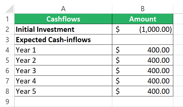
Seems promising. Investing $1000 in the first year, we get $400 in cash flows for the coming 5 years!
Nice – but the initial investment includes $400 from my savings (call it equity), and the other $600 is loaned by the bank. My cost of equity is 10%, and the interest rate I get to pay the bank is 12.5%.
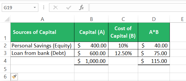
Turns out that the discount rate for this cashflow analysis must be an average of them both – more precisely, a weighted average of both the sources of my funds.
No big deal, here’s how we calculate the Weighted Average Cost of Capital (WACC) for this project:
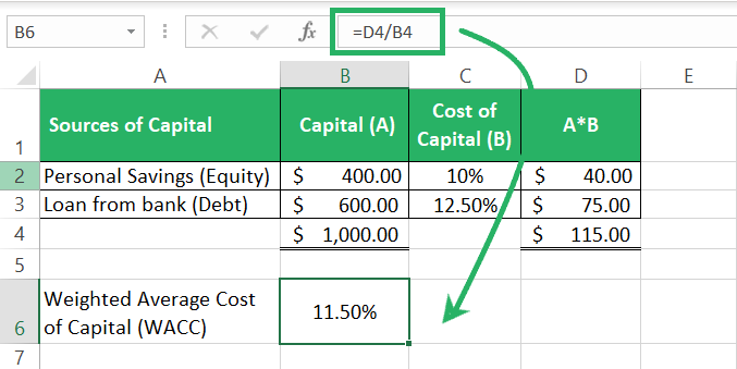
Okay, cool! Next, to find the NPV for this project:
Step 1) Begin writing the NPV function as follows:
Step 2) Refer to the rate as the first argument (the WACC we just calculated above)
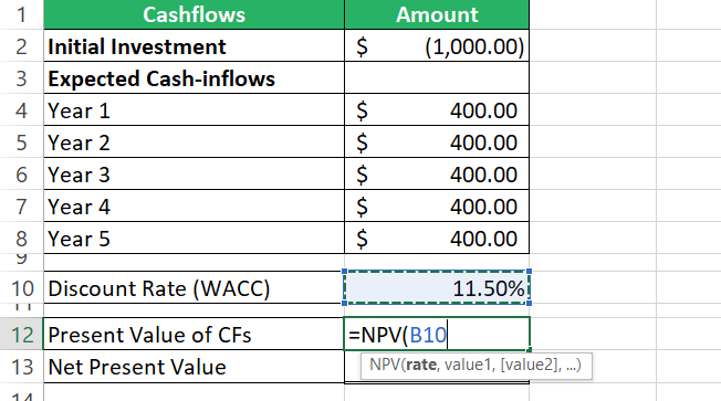
Step 3) And then, refer to the cell range that contains the cashflows to be discounted (B4:B8)
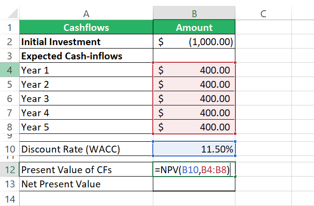
We are good – hit the enter key.
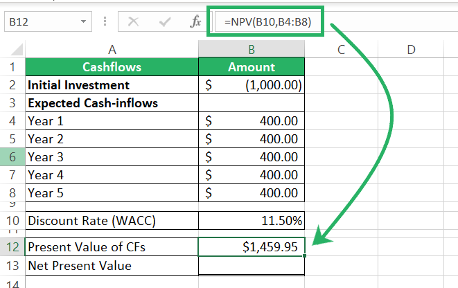
And there you have the present value for the given series of cashflow discounted using WACC.
Step 4) To know the Net present value of an investment, we deduct the initial investment outlay from it. See here:
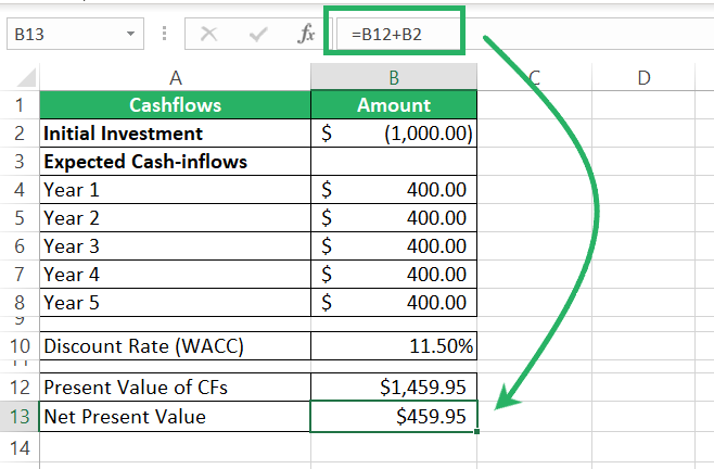
Since the initial investment is a cash outflow i.e., a negative value, we sum it up with the present value of the remaining cash inflows. Basically, we are deducting the investment from the present value of cash flows.
There you have it!
The NPV of this startup business is $459.95 😍
To break it down to easier terms, this startup earns you a net profit of $459.95 in today’s value of money.
How to check if Excel NPV is accurate
Running the NPV function is not the only way to come down to the net present value for a given series of cashflows in Excel.
You can also run a manually devised formula to do that. In this section, I will show you how can you calculate NPV in Excel manually.
And in the process, we will double-check if Excel calculated the right value or not 🏸
Plus Point: This section teaches you the math that runs behind the NPV function.
Aa ha – intriguing enough? Let’s go.
Step 1) To manually calculate NPV in Excel, write the following formula:
Our discount rate sits in Cell B10, so I am creating an absolute reference to it.
The number of years denotes the year in which the cash flow occurs. For example, for the 1st Year’s cash flow, it would be 1, for the 2nd Year’s cash flow, this would be 2, and so on.
For this, I am creating a relative reference to the year number in Cell B2.
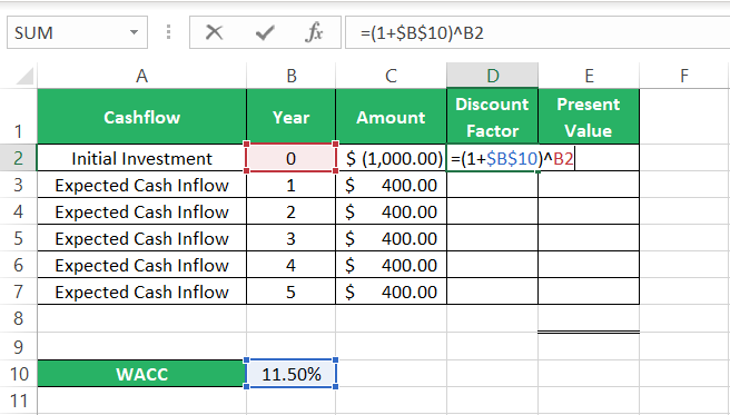
By Year 1, we mean the cashflow occurs at the end of Year 1. As the initial investment occurs on Day 1 (in other words the beginning of Year 1) – we take it as Year 0.
Step 2) Drag and drop the formula until the end of the series of cash flows.
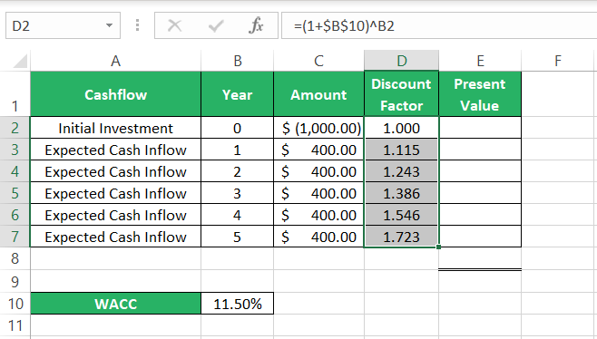
These, we call the discount factors.
Step 3) Next, divide each cash flow by its respective discount factor as below.
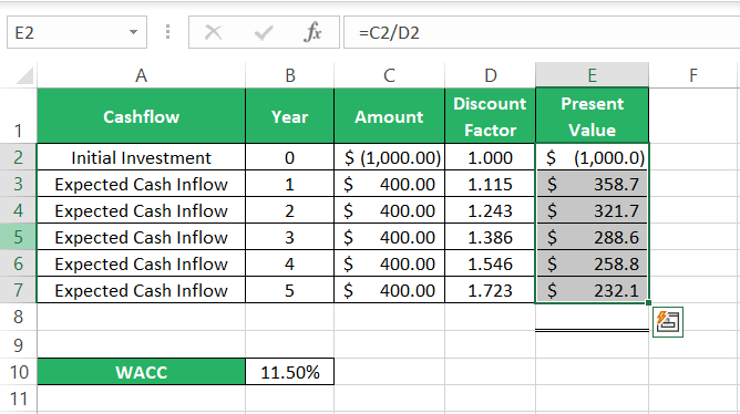
Step 4) And sum them all up!
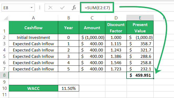
What a precise match to our example in the above section.
P.S: You do not need to double-check the results of the NPV function every time – keep calm and trust Excel 😄
NPV and IRR
IRR stands for internal rate of return. It shows the profitability level of any project.
In our example above, our WACC was 11.5%. This means, we bore a cost of 11.5% per annum to invest $1000 in the above project.
But how much annual rate of growth is the project earning us? IRR will tell you that.
Step 1) Write the IRR formula in Excel as follows:
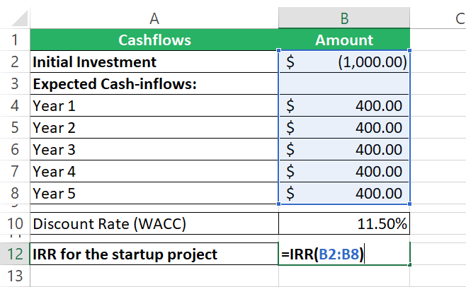
Step 2) Hit enter to have the IRR as 29%.
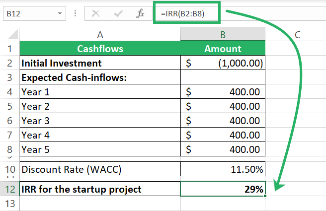
A 29% IRR means the project earns you back 29%. In other words, the NPV of this project when discounted at 29% would be zero 💡
See here:
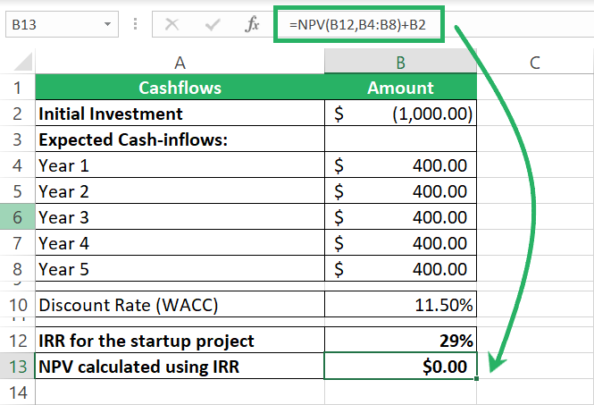
That’s the relation between NPV and IRR.
IRR is the discount rate that makes the net present value of a project zero.
In layman’s terms, you are paying 29% cost of your capital to invest in a project. And the project earns you back only 29%, what do you get out of it? Zero.
That’s what IRR says.
The higher the IRR of a project, the more the project is profitable.
NPV vs. PV vs. XNPV function in Excel
NPV is not the only function of Excel to calculate present values. There are two others as well. Here’s how they differ from each other.
NPV function
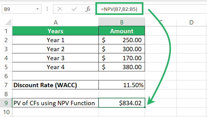
The NPV function calculates cashflows for varying cashflows that you can individually specify. Like here:
PV function
The PV function of Excel can calculate the present value only for a similar set of cashflows. The syntax for this function looks like below:
As the first argument, you give in the rate. Nper means the number of years over which the cashflows occur. And pmt denotes the cashflow. As pmt you can only enter a single cash flow say $100.
So, if you’re yielding $100 in cashflows for 10 years, here’s how it works:
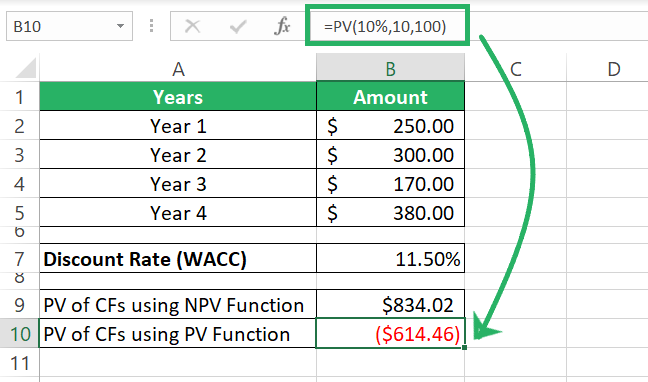
But if you have varying cashflows like $100 in Year 1, $200 in Year 2, $380 in Year 3, and so on, the PV function won’t be of help 📝
XNPV function
The NPV function is an advanced version of the NPV function where you can discount cashflows occurring on different dates, like below:
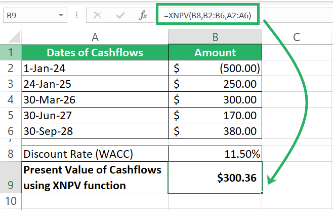
Not all cashflows would arise on year ends. The XNPV function comes in handy when you have cashflows occurring on other than a regular annual basis (irregular intervals).
Other Resources
I hope you found calculating NPV as interesting as I do.
Excel’s financial functions library has so many more similar functions for you to explore. Some of my favorite and most used functions from this library include:
Additionally, I have also covered some other key financial concepts like calculating Compound Interest in Excel and using the Amortization Calculator in Excel in great depth in my blogs here.
Give them a read, and let me know how you like them!
