How to Use the IRR function in Excel: Step-by-Step (2024)

IRR stands for Internal Rate of Return and originates from the field of finance.

IRR is crucially evaluated for the major financial decisions of any Company.

What is it? And how do you calculate it in Excel? 🤔

All of this and much more come your way as you continue reading the article below.

Download our free sample workbook here to practice the examples discussed below.

What is IRR?

The Internal Rate of Return (IRR) is the discount rate where the present value of future cash flows for any project equates to zero. Most of the time this is the interest rate at which the company would borrow for any project.

Financial experts would use it to assess the returns coming from different projects. And based on the same, investment decisions are made.

There is one crude way how you may calculate IRR manually (using a simple calculator). However, you can never get precise answers by solving IRR manually.

Only financial calculators and automated functions like the Excel IRR function can help you find a very precise IRR.

How to calculate IRR in Excel with the IRR function

How can you calculate IRR for a project in Excel? Take the data in the image below as an example.

The data above shows a series of positive and negative cash flows in Excel.

For example, you decide on starting a new project. It requires an initial investment of $5000. This initial investment (outgoing payment) is shown as a negative cash flow in Year 0 (today).

And the project will generate cash flows of $2000, $3000, and $4000 in each of the coming years, respectively. (Shown as positive cashflows in Years 1, 2, and 3).

1. To compute the IRR for the above data, write the IRR function as follows.

=IRR(B2:B5)

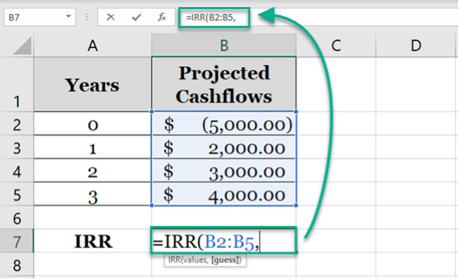
The first argument is ‘values.’ Create a reference to the series of cash flows (B2:B5) for the values argument.

2. In place of the second argument i.e. guess, enter an estimate of the expected IRR.

=IRR (B2:B5, 15%)

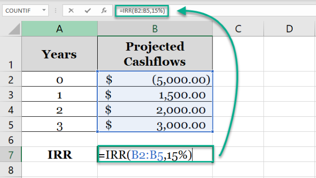
We have set it to 15%.

3. Excel calculates the IRR for the given cashflows as below.

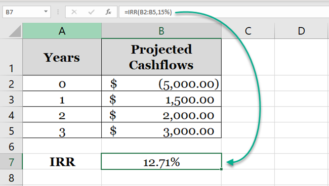
4. The IRR given by Excel is 12.71%.

Here’s something for you to note:

5. Even if you set the guess argument to a different percentage than 15%, the answer would remain unchanged.

Let’s set it to 19%, and the IRR would still be 12.71%.

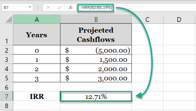
6. The guess argument is only an optional argument. It makes little difference to the result.

Pro Tip:

Often, the IRR calculated by Excel comes off as a round percentage (with no decimal positions).

This might indicate that the decimal positions are set to 0, and Excel has rounded up/down the IRR. To get a precise measure of IRR, increase the decimal positions.

Select the cell that contains IRR, and go to Home > Number > Increase Decimal.

IRR vs. NPV

How can we check if the IRR calculated by Excel is accurate?

You may cross-check it by quickly applying the NPV function.

NPV stands for Net Present Value. When the projected cashflows for a project are discounted and summed, the result is NPV.

Pro Tip!

The higher the NPV, the better. Similarly, the higher the IRR, the better.

In simplest terms, a positive NPV gives the ‘Go Ahead’ for undertaking a project. A negative NPV indicates that a project must not be undertaken.

IRR, whereas is the discount rate, where the NPV for a given set of cashflows would be zero.

So, to check if the IRR for a series of cashflows is correct, run the NPV function to see if the NPV turns out to be zero.

1. For the IRR calculated above, write the NPV function as follows.

= NPV (B7,

Cell B7 contains the IRR for the cashflows above. We have created a reference to Cell B7 as the first argument.

2. Write the second argument for the NPV function.

= NPV (B7, B2:B5)

The second argument requires values (cashflows). We have created a reference to cell range B2:B5 that consists of the cashflows.

3. Hit Enter to see the results.

The NPV is zero. This vouches for the IRR to be accurate.

If you get a positive Net present value or a negative one, you are likely to have landed on the wrong IRR.

Common errors when calculating IRR

Until now, you must’ve found the IRR function to be a piece of cake. However, some conceptual issues may arise with the IRR function.

These can cost you the wrong IRR or an error from Excel. Look at each of them below.

1. Blank Cells in the Value argument

1. If your cashflows look like this:

The image has a series of cashflows starting from Year 1 to Year 5. However, the cashflows for Years 2 and 4 are zero. So, the relevant cells are left empty.

2. Now, if you apply the IRR function as follows:

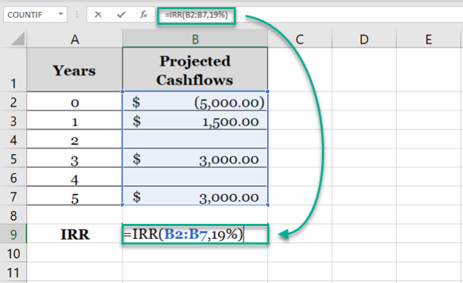
The IRR would be 20.79%.

Replace all empty cells with zeros and reapply the IRR function as below.

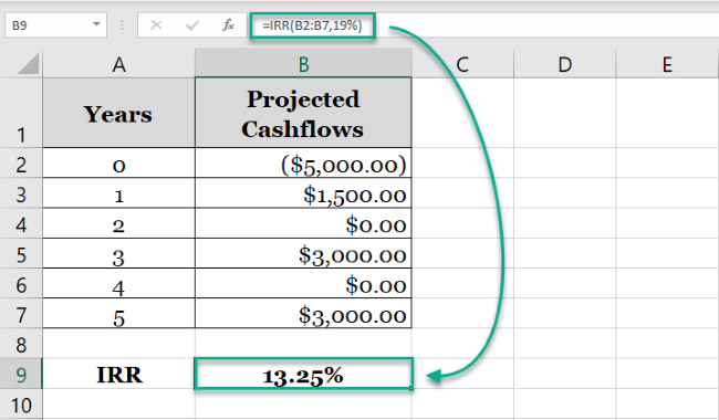
IRRs for both datasets show a dramatic difference. 20.79% to 13.25%.

This is because the IRR function doesn’t count in empty cells.

So, if your cashflows show zero cash flow for any year, make sure it is zero and not left blank.

2. Uneven Intervals

What if you get monthly cash flows from your project after three months, then after six months, then after one year, and so on?

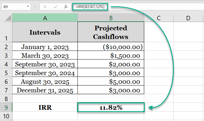
With such a dataset, if you apply the IRR function, the results would not be accurate.

This is because the IRR function assumes that all cash flows occur at regular intervals.

If you have cash flows that occur at different intervals, as shown above, you may use the XIRR function.

Pro Tip!

The IRR calculated by Excel is the rate per interval. What if the cashflows in your dataset occur at different intervals (say every three months) but you want the IRR per to be annum?

Calculate IRR as explained above, Once found, use the formula below to convert the IRR from the rate per quarter to the rate per annum.

= (1 + IRR) ^ 4 ) – 1

Why 4? The interval here is of three months, and 12 months divided by 3 months is 4.

3. The NUM Error

Applied the IRR function, but all that Excel returned was a NUM Error.

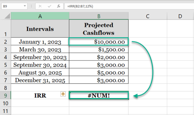
Double-check if the series of cashflows contain at least one negative and one positive value.

That’s it – What’s next?

That’s all about the very easy IRR function of Excel. It only takes two arguments and is effortless.

This article teaches you the basics of IRR, and how the IRR function may be used to calculate IRR in Excel.

It also explains how IRR is different from the Net Present Value. And how you may counter the problems that the IRR function may pose.

You can take your finance career to a next level using these smart functions offered by Excel. However, this is only possible when you use these functions together with other major functions of Excel. 👍.

These functions include the VLOOKUP, SUMIF, and IF functions. My free 30-minutes email course is all that you’ll need to get the hang of these functions (and many more).

Other resources

Had a good learning experience here? We have tons more articles that’d help you explore the financial functions offered by Excel.

Hop on here to learn about the PMT function of Excel. Or automate your loan calculations by developing a loan calculator in Excel.