How to Print an Excel Spreadsheet on One Page (+ More)
Trying to fit your big spreadsheet into 1 tiny page?
As easy as it seems, printing Excel spreadsheets can be difficult if you don’t know the pro tricks. And even more so if you’re new to this software.
Luckily, this guide has everything you need to know about printing Excel spreadsheets. We’ve jotted down some of the most important Excel techniques to help you get started 😃
So without further ado, let’s get right into it.
Also, if you want to practice along the guide, download our sample workbook here.
Table of Contents
How to print an Excel sheet on one page
Sometimes we just want to squeeze all our data on one page to avoid extra mess. But by default, Excel prints multiple pages for data that can easily show up on a single page.
Not only does this lead to wastage of paper, but managing so many hard copies can be a true hassle.
This is why people prefer accommodating most of their data on a single page. And if you don’t have extensive data or readability issues, this is the ideal approach.
Let’s suppose we have some data set, and we want to print it on one page 📄
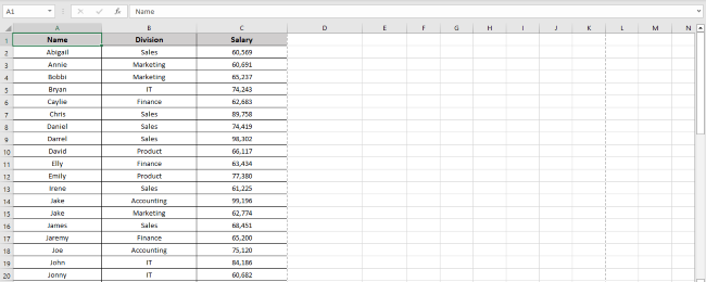
So to print the Excel sheet on one page:
- Click Print from the File Tab.
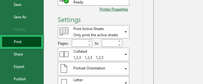
- The Print Preview screen shows up.
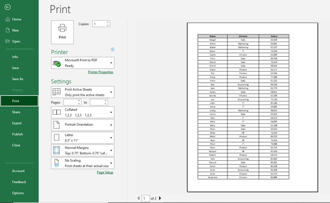
The Print Preview screen gives you an idea of how your data will look on a printed page. Our printed page is in Portrait orientation and spread over two pages.
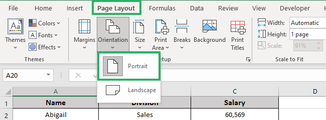
If you prefer, you can change the page orientation from the print settings shown above. Or the Page Layout Tab from the ribbon.
If you have columns to print, choose Landscape. And if the data consists of more rows (like in our case), choose Portrait.
To fit all the rows on one page, we will scale it accordingly.
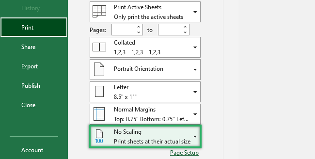
- Click the ‘No Scaling’ option at the bottom.
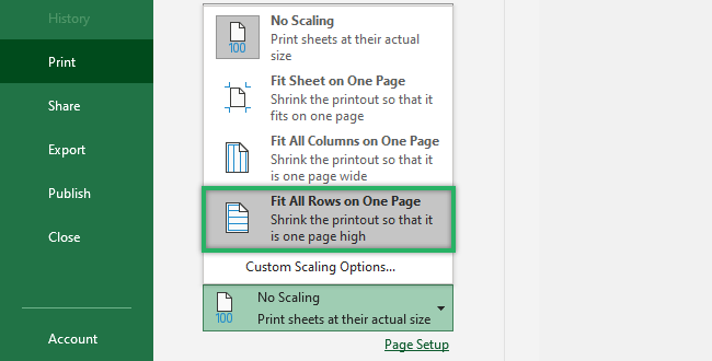
- Select ‘Fit All Rows on One Page.’
- Excel shows the preview as:
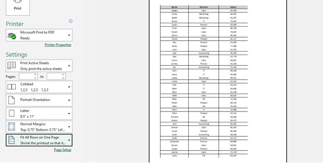
All your data will now be printed on a single piece of paper 📝
Note that scaling an Excel sheet on one page can make the printout hard to read.
How to print the entire workbook
We just saw how to print the Excel spreadsheet on a single page. Now, let’s see how to print the entire workbook in one go.
It’s quite straightforward. All you need to do is:
- Go to ‘Print” from the File Tab.
- `Click ‘Print Active Sheets’ in the Print Preview area.

- Select ‘Print Entire Workbook.’
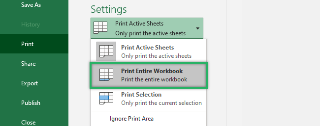
Excel will now print the entire workbook when you click Print.
Pro Tip!
You can select other options too. For instance, if you only want to print a specific selection in the sheet, click ‘Print Selection.’ And if you want to print the Excel worksheet, select the ‘Print Active Sheets‘ option.
How to change the print area
As evident from the name, the Print Area lets you choose a specific portion of the spreadsheet that you want to print.
This is because often, we don’t want to print the entire sheet but only some part of it. The Print Area feature can help you do just that. And its working is similar to that of Print Selection under the Print Settings.
To enable the Print Area:
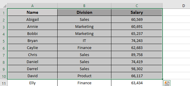
- Select the data you want to print.
We want to print the first ten rows of our data set:
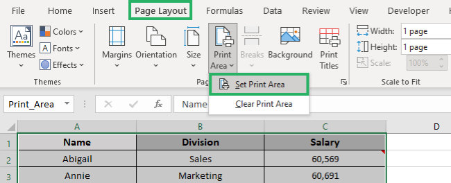
- Go to the Page Layout Tab.
- Select Print Area under the Page Setup group.
- Click ‘Set Print Area.’
And it’s done! 🥳
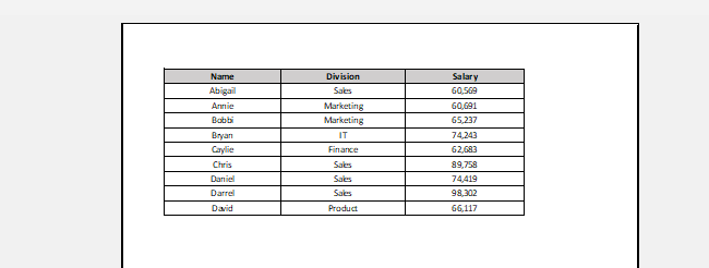
Excel will now only print the selected data. You can view the Print Area in the Print Preview window as well 🗔
Pro Tip!
You can also choose whether you want to show the gridlines for printing or not. For that, select the ‘Print’ option under Gridlines from the Sheet Options group.
Excel will now print the gridlines as well. You can view them from the Preview window.
You can also add a new print area to your previous selection. All you need to do is select the new range and press Print Area.
Then select the ‘Add to Print Area’ option.
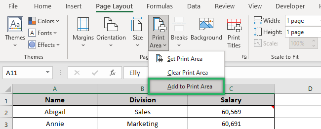
The selected portion is now added to the Print Area 📃
Similarly, if you want to remove it, click Clear Print Area. Excel will remove the entire Print Area.
How to print comments
If your comments are just as important as your worksheet data, know that you can print them too. The process takes a few seconds only and is easy to understand 😃
To print Excel comments:
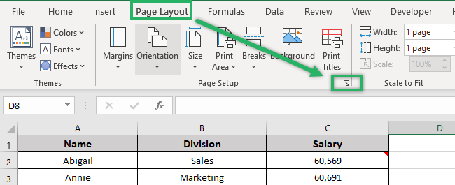
- Go to the Page Layout Tab.
- Open the Page Setup dialog box (from the small arrow at the right corner)
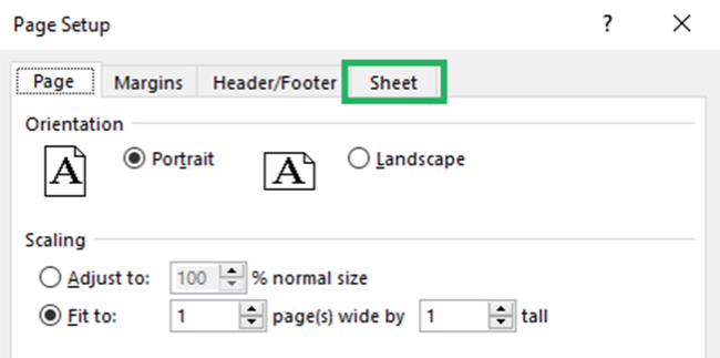
- Click the Sheet tab.
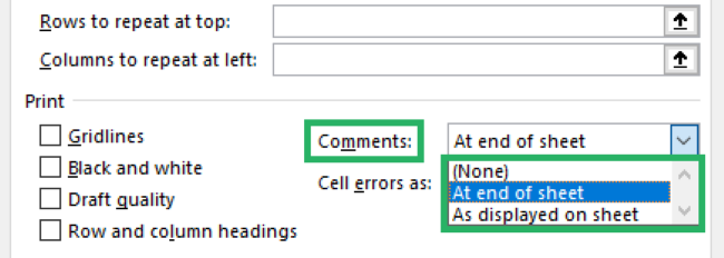
- Click the drop-down arrow next to Comments and select an option.
- Press Ok.

You can now see how the comments will appear on paper in the Print preview window 📄
Just scroll down or move to the next page to view them.
That’s it – Now what
Printing spreadsheets in Excel can be tricky, especially when you have large data to print. But using these new techniques, you will be able to wind that hours-long task in minutes.
Summing up, we learned how to print an Excel sheet on one page in this article. We also saw how to print comments, the entire workbook, and even change the Print Area.
Knowing how to print Excel spreadsheets is pretty important when working in a professional environment. But so are the other things in this giant spreadsheet software that you need to learn!
If you are just starting out, we recommend you practice the Excel VLOOKUP, IF, and SUMIF functions. Enroll in my 30-minute free email course that teaches these functions and much more for FREE! 😵
Other resources
These printing tips and tricks are sure to give a boost to your Excel skills. All you need is constant practice and more knowledge.
If you enjoyed this article, we’re sure you’d love to know more. Try reading How to Print Gridlines, Mailing Labels, and more.
