How to Use the RATE Function in Excel (Interest Rate)

Life is all about decisions and half of these are financial decisions.

The RATE function of Microsoft Excel is designed to help you with these financial decisions as it calculates the interest rate implied in an arrangement in seconds ⌚

Interested to see how? Grab your free practice workbook for this guide here and continue with me till the end.

Table of Contents

What is the RATE function

The RATE function of Excel is a financial function that finds the rate implicit in an arrangement.

For example, you enter into a loan agreement with a bank where the bank pays you $500 today and you pay it back in equal installments of $250 per year for 3 years.

You are paying back more than what you borrowed – $500 vs. $750 ($250 * 3 years). So, you know you’re paying some interest on the loan. But how much percent interest? 💰

The RATE function calculates it for you.

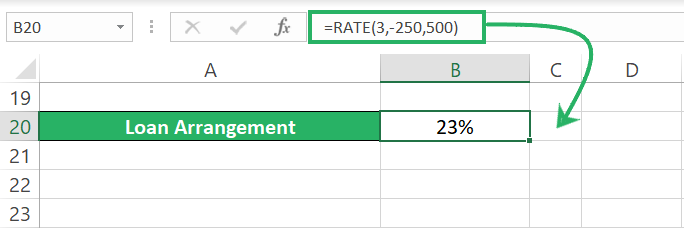
The RATE function works on a trial and error (iterations) method and can return multiple results or no result at all.

Syntax

The syntax of the RATE function is as below:

Where:

• Nper (required argument) – the total number of payment periods
• Pmt (required argument) – the constant amount of payment per period that cannot be changed over the life of the annuity. Can be omitted if you give the FV argument.
• Pv (required argument) – the present value of the loan or investment, i.e. the current value of the loan or investment. Can be omitted if you give the FV argument.
• Fv (optional argument) – the future value of the deposit/loan/investment. If omitted, it defaults to 0. Becomes mandatory if the PMT or PV argument is omitted.
• Type (optional argument) – indicates when the payments are made:

0 or omitted – payment is made at the end of the period

1 – payment is made at the beginning of the period

• Guess (optional argument) – your guess for what the rate might be. If omitted, Excel assumes it is 10%.

Pro Tip!

The RATE function works on a trial-and-error method. If would try different rates that fit the given arrangement and return the answer after 20 iterations.

However, if it fails to converge to a rate even after 20 iterations, it results in the #NUM! error ❌

The guess argument is optional and can be omitted most of the time. However, sometimes doing so might result in the #NUM! error if Excel fails to converge to a rate after 20 iterations.

Giving in a guess rate helps Excel start conversions closer to this rate converging to the correct answer within 20 iterations. Use a guess rate other than 10% (it is assumed by Excel by default).

Using the RATE Function of Excel

Let us now see through multiple examples how to use the RATE function of Excel to calculate the interest rate/rate of return in Excel.

Series of Payments

If you are making periodic payments, there can be two possible ways how you’d want the RATE function to work for you.

Example 1: (Pmt and PV)

The first instance is where you have the present value and periodic payments known and want to find the rate for it.

Suppose you rolled out a loan of $1000 from the bank against yearly payments of $300 for 4 years. What is the interest rate borne by this loan? ⁉

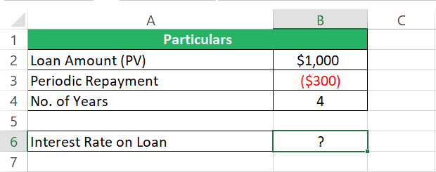
You know the present value of the loan ($1000) and the periodic payments to be made against it ($300 per year). Let’s now find the interest rate implicit in it.

Step 1) Begin writing the RATE function.

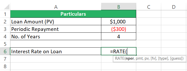
Step 2) As the nper argument, give the number of years for loan repayment.

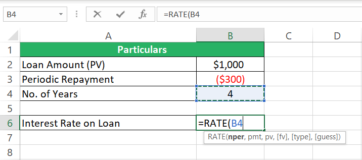
Step 3) As the pmt argument, we will refer to the periodic future payments of $100 to be made over 4 years.

Pro Tip!

Very important to note that cash outflows should appear with a negative sign (like the periodic payments).

And cash inflows should appear as a positive number (like the loan received by us). If both the values are positive or negative, the RATE function will return a #NUM! error.

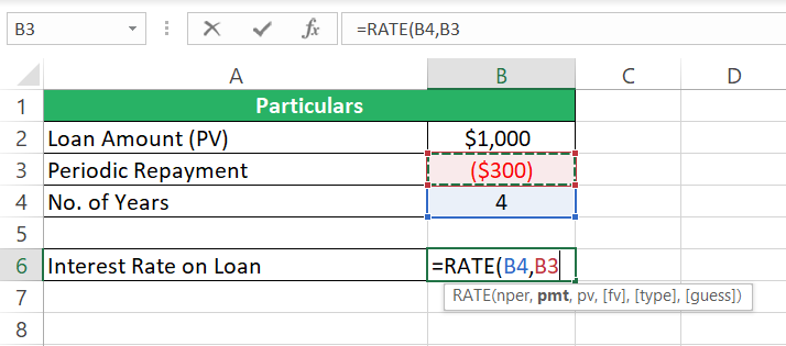
Step 4) As the pv argument, refer to the amount of loan received from the bank.

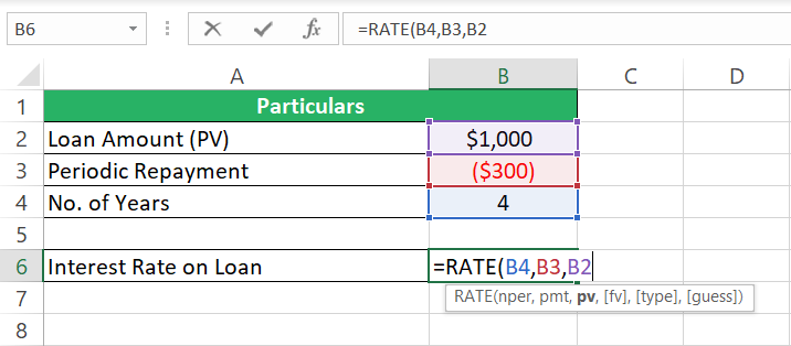
Step 5) We don’t know the future value of this arrangement. Omit the fv argument.

Step 6) Assuming the loan payments are made at each period end so omitting the “type” argument.

Step 7) The guess argument is also optional so omitting it too.

Step 8) Press enter to have the interest rate calculated.

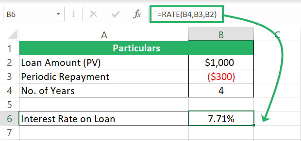
Excel returns 7.71% as the interest rate implicit in this loan arrangement.

Pro Tip!

The nper and the guess arguments must be coherent. For example, if you are making monthly payments for two years, your nper argument would be 24 (2*12).

Accordingly, supply the guess argument as a monthly rate (if you guess it to be 12% annually, supply it as 12%/12 = 1%.

Here’s another catch – the RATE that Excel would calculate for you would also be coherent with the nper supplied by you. If you have supplied it for quarterly payments, Excel will return the quarterly rate.

Example 2: (Pmt and FV)

This example is about a situation where you know the periodic payments and the future value but not the present value.

Suppose you make periodic payments of $200 each year for 4 years to your savings account and at the end of Year 4, your savings account pays out $1000 🏦

So you know the periodic payments ($200 each year) and the future value ($1000) at the end of year 4.

What rate of return is your saving account paying? Let’s find out.

Step 1) Begin writing the RATE function.

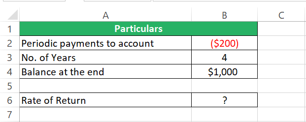
Step 2) As the nper argument, give the number of years over which you’ll make periodic payments to the saving account.

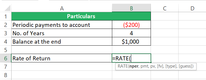
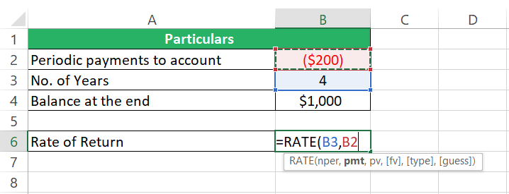
Step 3) As the pmt argument, we will refer to the periodic payment of $100 to be made over 4 years.

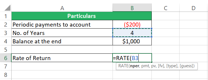
Note the periodic payments come as negative numbers since you’re paying them (cash outflows). The balance in the account at the end of 4 years comes as a positive value since that is what you receive from the bank at the end of the annuity (Cash inflow).

Step 4) We don’t know the present value for this example so we will leave the pv argument omitted.

Step 5) As the fv argument, supply the future value of this account (at the end of the annuity period).

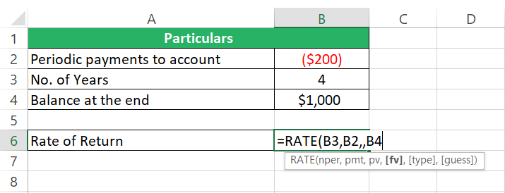
Step 6) All done. Hit down the enter key to find the rate of return paid on your savings account.

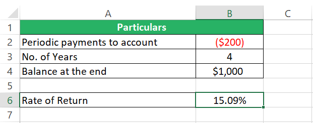
That’s 15.09% per annum 🤩

Lump Sum Payment

This section deals with finding the rate of interest/growth when there are no periodic payments but a single lump sum payment.

For example, I invested $100 in a company 3 years ago. Today my investment stands at $300. At rate per year did my investment grow?

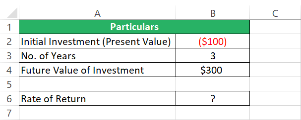
You know the present value ($100) and the future value ($300) of your investment. Let’s find the rate of growth now.

Step 7) Begin writing the RATE function.

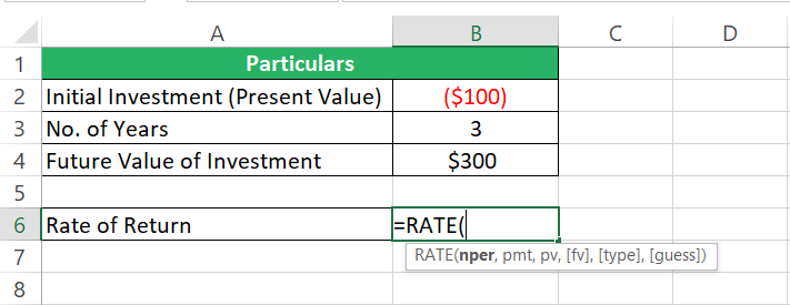
Step 8) As the nper argument, give the number of years over which the investment has grown.

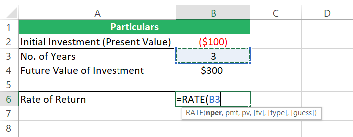
Step 9) Since there are no periodic payments, omit the pmt argument.

Step 10) As the pv argument, refer to the initial investment. This is where the investment started growing.

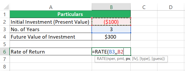
Step 11) As the fv argument, refer to the future value of the investment at the end of Year 3.

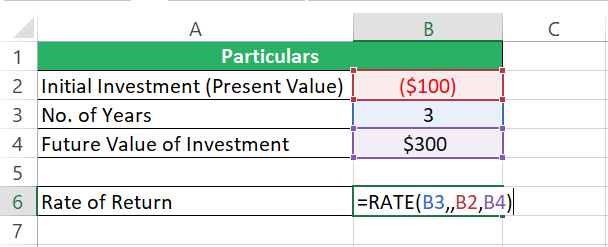
Step 12) Press enter to have the rate calculated.

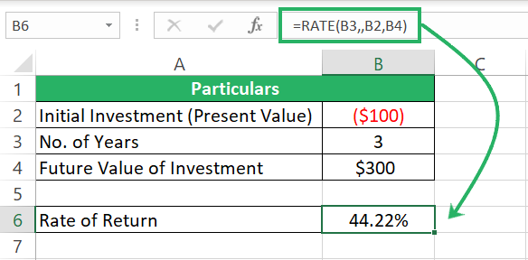
That’s 44.22%%. This means that your investment grew by 44% each year 🎯

Step 13) If you apply a 44.22% growth rate to the investment of $100, you get $144 by the first year-end.

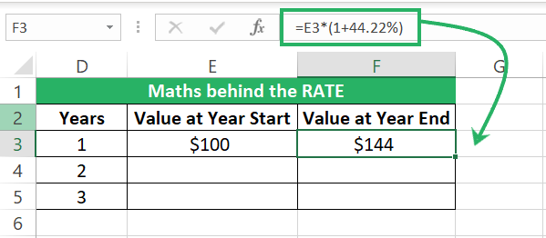
Step 14) Compound $144 on 44.22% for another 2 years to get $300 by the end of Year 3.

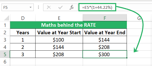
The RATE function tells that if you grow your investment of $100 will grow to $300 in 3 years, if compounded on 44.22%.

Conclusion

The RATE function is an important financial function of MS Excel that is widely used by investors, banking professionals, and others from the domain of finance.

Learn more about other financial functions of Excel by reading the exploring the following Excel tutorials of mine.

• How to Use Excel’s Annuity Formula (Example)
• How to Calculate Present Value (Excel PV function)