How to Fix the #Ref Error in Excel (Step-by-Step)

Often it is the case that everything looks good about your spreadsheet. But then you delete a row or a column to make some final touches.

And suddenly half of your spreadsheet goes crazy with the #REF error🥴Why does this happen? And what does it mean?

The #REF error of Excel is the short form of Reference. It appears when one or more of the cell references in your spreadsheet turn invalid.

The guide below will teach you everything about diagnosing and fixing #REF errors in Excel.

So continue reading. And as you scroll down, download our sample workbook here to tag along with the guide.

What causes the #ref error

#REF error is Excel’s way of saying that the cell reference for this formula is no more valid.

This would happen when these cell references have either been moved, deleted, or overwritten ✂

Check this out:

In the image above, we have added up a few cells, and everything seems good.

Delete one of these cells (say cell A3) and see what happens.

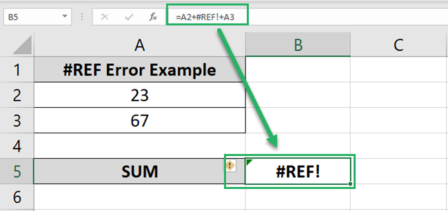
The formula says = A2 + A3 + A4.

And as we delete cell A3, we have no more valid references. The cell reference for the deleted cell goes invalid and this results in a #REF error😵

Additionally, you might see the #REF error in Excel when you copy a formula with relative references.

See here.

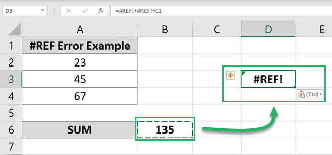
We have copied the formula = A2 + A3 + A4 from Cell B6 to another cell in Excel.

As the formula has relative references, Excel updates the cell references for its new position. And as nothing sits in place with the updated cell references, we get the #REF error.

#REF error might also occur when a sheet of your workbook bears a link to cells from another sheet, and you delete that sheet.

How to fix the #ref error

We’ve now seen the reasons why the #REF error might occur in Excel. Let’s now jump into the solutions to these errors.

Use In-Built Excel Functions

Here’s the simple addition example that we saw only in the previous section:

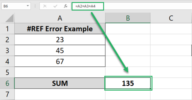
Instead of writing the formula = A2 + A3 + A4 had you used the SUM function, the results would’ve been different 🌟

Check out here:

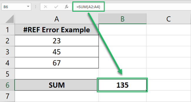
Instead of using the “+” operator, we have applied the SUM function to add up the numbers.

Now, if you delete Row A3 altogether, this is what happens 👀

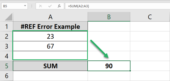
No more #REF errors. The SUM function automatically adapts the cell references and changes the formula to = SUM (A2:A3)

And so, most of the time when operators would land you into errors, Excel functions might save you 🦺

Do not delete linked rows/columns/sheets

Do not delete rows, columns, or sheets that might bear references to any of your formulas.

This might delete the abundant data from your spreadsheet. But your formulas would go crazy.

If you delete a row, a column, or a worksheet and you get the #REF error, don’t lose your calm already 😩

There are two ways how you may fix this:

1. Hit ‘Control + Z’ to undo your last action. This will restore the deleted cells, and all your formulas will come back to life.

Search for the data that’s still relevant to your formulas, and do not delete it.

2. Remove the cell or range reference from your formulas and use simple values before you delete any abundant data.

You can do this by copying formulas and pasting them as simple values📃

Do not copy formulas with relative references

Remember what happened when we copied the formula from one cell to another?

The cell references in the formula (A2, A3, and A4) were relative references. As the formula changed place, Excel updated the cell references which resulted in a #REF error.

You can help with this as follows:

1. Select the cell containing the formula.
2. Click on a cell reference (say A2) and press the F4 key.

This will convert the formula into an absolute reference.

3. Do this for every cell reference.

Your formula must look like below:

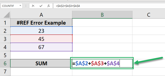
4. Press “Enter” and you’re good to go.

Try copying/pasting the formula to a different location now 🤩

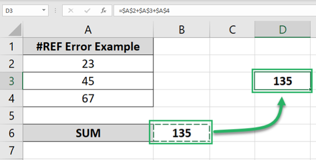
When converted into absolute references, cell references do not change when the formula is moved.

So the results remain consistent, and you get no more #REF errors.

Examples of formulas that return the #ref error

Let’s now look into some common formulas that return the #REF error when misapplied. Check it out here.

Example No. 1: VLOOKUP function

The VLOOKUP function searches for a value in a given range of data. Once found, it returns any value associated with it from any corresponding column reference.

So let’s try using it in Excel 💪

Here we have the scorecard for some students:

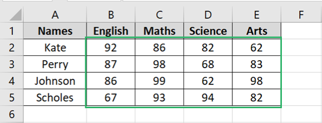
Can we readily find the marks scored by Perry in Arts? For that we must apply the VLOOKUP function as follows:

=VLOOKUP(“Perry”, A2:E5, 5)

We have told Excel to look for Perry in the table range from A2 to E5. And return the corresponding value for Arts from Column 5 (the col_index_num is 5).

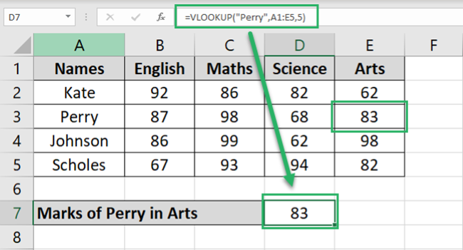
Perry scored 83 in Arts. Wow, she must be a good artist 🎨

But what if you mistakenly input the col_index_num as 6 instead of 5 in the above example?

Here’s what will happen.

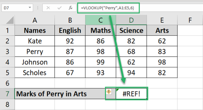
Excel returns the #REF error. That’s because there is no column 6 to the specified data range. There are only 5 columns.

Excel fails to understand which value must be returned. And hence the VLOOKUP function returns the #REF error 🚩

Example No. 2: INDEX function

Just like the VLOOKUP function, the INDEX function also returns a specified value from a given array.

How? Check out here:

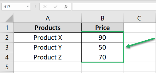
The image above has the price of some products.

Let’s use the INDEX function to find the price of Product Z.

=INDEX(A1:B4,5,2)

This tells Excel to look to return the value from Row 5 and Column 2 of the data range A1:B4.

Here’s what we get:

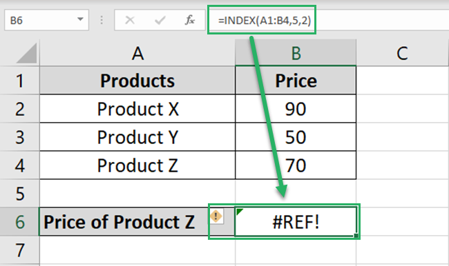
Oops! A reference error ❓

Guess we did something wrong. We mentioned Row 5, but the data range A1:B4 has four rows in total.

Excel fails to find Row 5 in the specified date range and returns the #REF error.

Let’s redo the INDEX function as follows:

=INDEX(A1:B4,4,2)

We have only changed the Row number to 4 (where Product Z lies). And the results come out as follows:

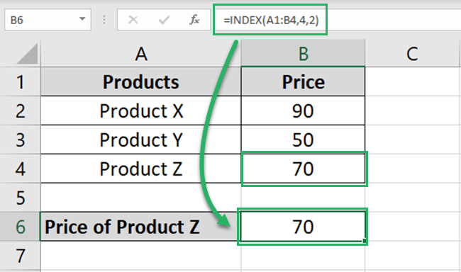
We have landed on the right figure. Product Z is priced at a whopping $70.

Non-existent row/column numbers can cause the INDEX function to return the #REF error.

That’s it – Now what

That’s all about the #REF error in Excel. You now know what causes the #REF error in Excel and you can fix it too, can’t you 🔧

In the guide above, we have also seen multiple examples of formulas that might return the #REF error.

Hope you enjoyed learning. If you did, don’t just stop here. There’s just so much more to Excel that you must know. Like the nearly endless functions of Excel.

If you are on a mission to become an Excel maestro, make sure you are great at some of the basic Excel functions. Like the VLOOKUP, SUMIF, and IF functions of Excel 🚴‍♀️

To learn them (and much more about Excel), enroll in my 30-day free email course now.

Other resources

Excel errors are always undesirable. You can check if any of the formulas of your spreadsheet are erroneous using the ISERROR function.

And using the IFERROR function, you can even replace these errors with any other value.

Frequently asked questions