How to Remove Apostrophe in Excel – Before a Number
In Excel, we sometimes see numbers with leading apostrophes (‘).
Inserting a leading apostrophe in Excel will keep the leading zeros of a number.
However, there are times when Excel will display an unnecessary apostrophe. This is very common when you copy and paste numerical values or tables from web pages.
In this Excel lesson, you will learn two simple techniques for removing all the leading apostrophes from numerical data in Excel.
Let’s go!
Table of Contents
Remove apostrophe with Text to Columns Wizard
Most of the time, you’ll need to remove apostrophes while keeping the data in the same column.
To remove leading apostrophes in numbers, you cannot use the Search and Replace tool🤔
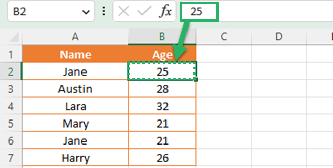
The reason for this is that, while you can see the apostrophe in the formula bar, it is not part of the cell content.
A number’s leading apostrophe is just a prefix character.
In this case, you can make use of the Text to Columns tool😍
All of the numbers in the table below contain a leading apostrophe.
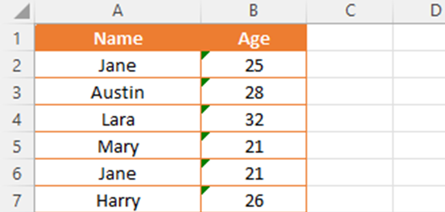
You can follow the below steps for that.
- Select numbers with leading apostrophes. In this example, you have to select cells B2 to B7.
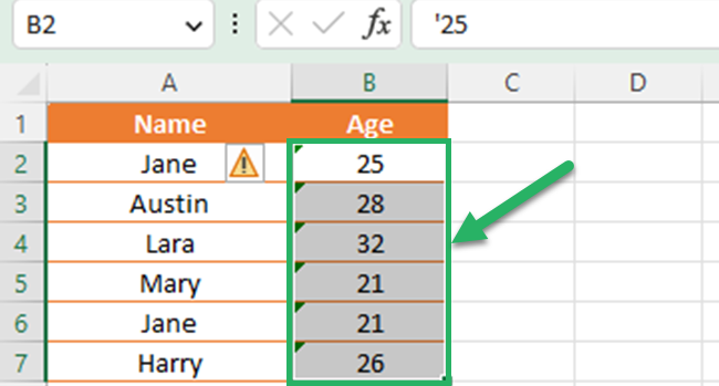
- Go to the Data tab and click the Text to Columns from the data tools group.

- Select the radio button of “Delimited” in step 1 of the Text to Columns wizard.

- Next, select the apostrophe (‘) as the text qualifier.
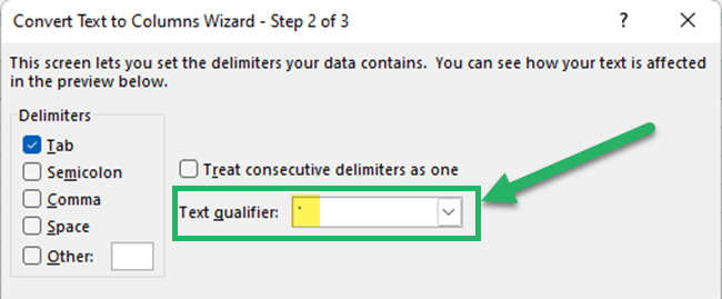
- Click the “Finish” button.
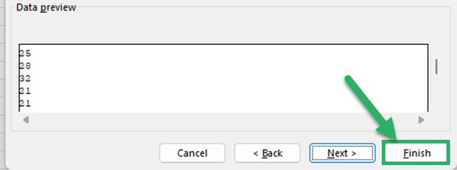
Then, you will notice that leading apostrophes are removed from all the cells👏🏻
Remove apostrophe with paste as values
Sometimes you need to get numbers to another column without leading apostrophes in those numbers🙂
Then, you can use paste options for removing apostrophes.
In the first table below, all the cells have an apostrophe before numeric values.
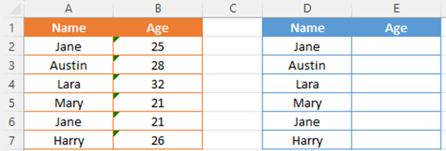
Now, you need to copy cell values in column B to column E without leading apostrophes.
You can simply follow the below steps for that.
- Select the data range that you need to copy.
In this example, you need to select cell values in cells B2 to B7.
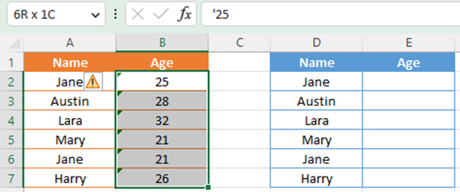
- Copy the selected cells. You can use the “CTRL + C” shortcut or select the “Copy” icon from the Home tab.

- Select cell E2 and expand the paste options.
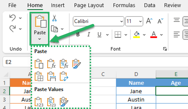
- Paste the copied cell data using the Paste Value option to the destination cells.
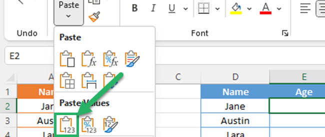
This method works only if you copy and paste numeric values to a new column⚠️
If you paste the values to the same data range (selected range with leading apostrophes), you will not get the desired result.
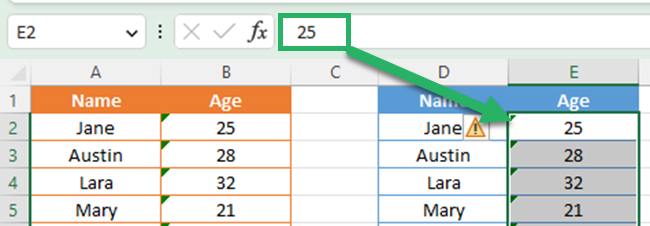
When you follow the above steps, you will get the same numerical values in column E without apostrophes🥳
If you check the formula bar, you will see there is no apostrophe before the numeric value in each cell.
Pro Tip:
You can do the paste values using the following methods also.
- Using the keyboard shortcut
ALT + H + V +V
- Using the keyboard shortcut to open the paste special options dialog box.
CTRL + ALT + V and then press again V.
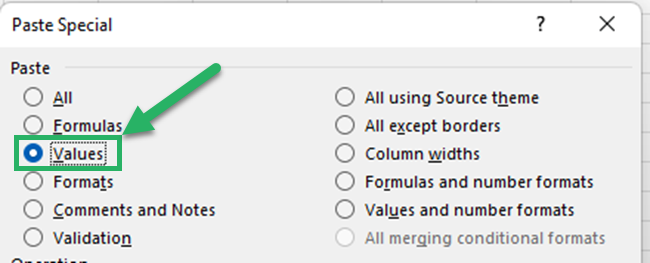
- Right-click on cell E2 and press V.

That’s it – Now what?
You now know how to remove apostrophe in Excel. Easy, right? 👍
There are many other methods to remove apostrophes in Excel such as using the VALUE function, clear formats, “convert text to number” etc.
Do you know that you can also write a VBA code in the module window to get the same numeric values without leading apostrophes?
You can quickly open a VBA module code window and enter a VBA code to remove leading apostrophes in your Excel worksheet.
New to VBA? 🤔 I got you.
Get started with VBA when you sign up for my free 30-minute online course (for beginners).
I promise you, it’s not as hard as you think🙌
Other relevant resources
This article helps to learn how to remove apostrophes in Excel.
We have other Excel tutorials to teach you how to remove unwanted things from Excel.
You can read our articles to learn how to remove extra spaces in Excel, how to remove dotted lines in Excel, how to remove blank rows in columns, and many more.
