If Cell Contains Text Then Return Value in Another Cell
Excel is a very smart spreadsheet software. And if you’re not using it to automate your tasks smartly – you’re not doing it right.
One of the major uses of Excel is to conduct efficient searches. Like searching for a specific text or just text in Excel and returning another value elsewhere 🧐
This process (if successfully worked out) can simplify your routine Excel jobs by multiple folds. In this tutorial, I will show you multiple aspects of how you can do it in Microsoft Excel.
Get your free practice workbook for this tutorial here and continue reading.
Check if the cell contains text
Here is a list of some values in Excel (a mix of text and numeric values 🔢).
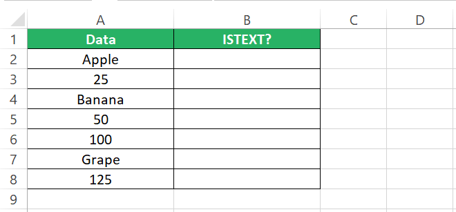
Which ones of these are text values, and which are otherwise? I know you can tell that just by seeing but this is because the dataset is not that huge.
As the data grows in size, identifying text values by merely scanning data might not be as easy as that.
How can Excel identify if a cell contains a text value or not?
By using the ISTEXT function – see here.
Step 1) Begin writing the ISTEXT function as follows:
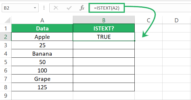
It returns a Boolean value (True or False) based on whether the given value is a text, or not.
Step 2) Drag the fill handle to get results for the whole list.
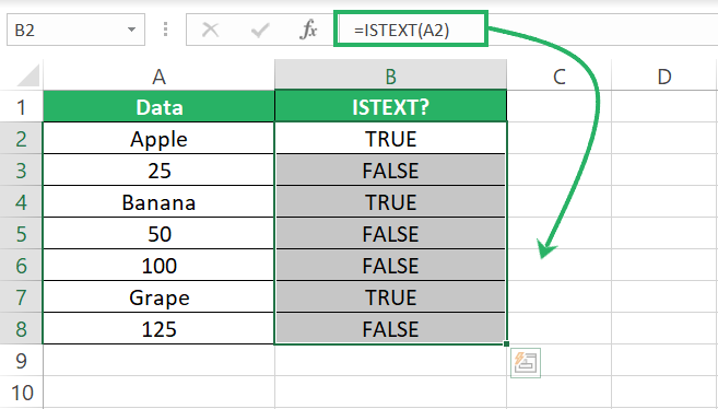
That’s how you can check if a cell contains text or not. But this doesn’t stop here.
Once you have checked if a cell contains text, you might want Excel to give back a certain value. This can be done by wrapping the ISTEXT function in the IF function.
Step 3) Nest the above function in the IF function as done in the following formula.
Step 4) Write the value that you want Excel to return if the cell contains a text value as the value_if_true (the second argument).
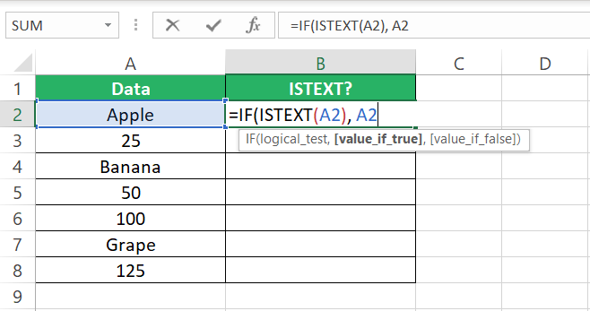
I want Excel to return the text value itself, so I have specified the cell (A2) that contains the value as the value_if_true.
Excel will only return this value if the ISTEXT function returns TRUE.
Step 5) Write the value you want returned if the cell doesn’t contain text as the value_if_false.
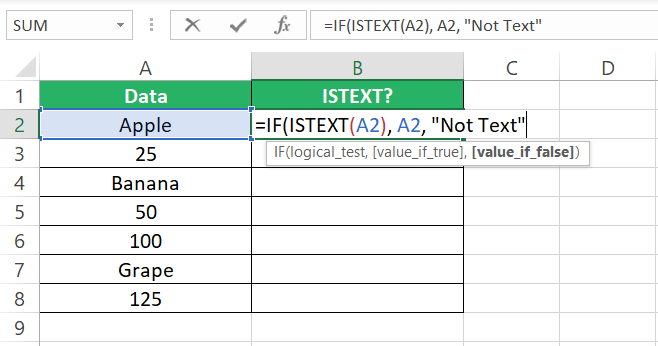
Can be anything, or you could also just omit it.
Step 6) Hit enter and drag the formula down to get the following results.
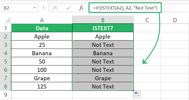
See that? For cells that contain a text value, Excel has returned the text and for those that contain any non-text value Excel returns the supplied value_if_false 🤩
Check if the cell contains specific text
Besides checking if a cell contains a text or non-text value, you might want to check if a cell contains a specific text.
For example, I have a list of students and their groups below 👩🏫
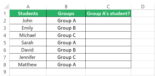
I want to see which of these are from Group A. For those who are from Group A, I want Excel to return “Yes” and for those who are not, “No”.
Step 1) Begin writing the IF function.
Step 2) Write the logical test as the first argument in the below formula.
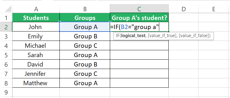
Just instructed Excel to check if the value in Cell B2 is Group A, or not.
Step 3) Give in the value_if_true as “Yes” and the value_if_false as “No”.
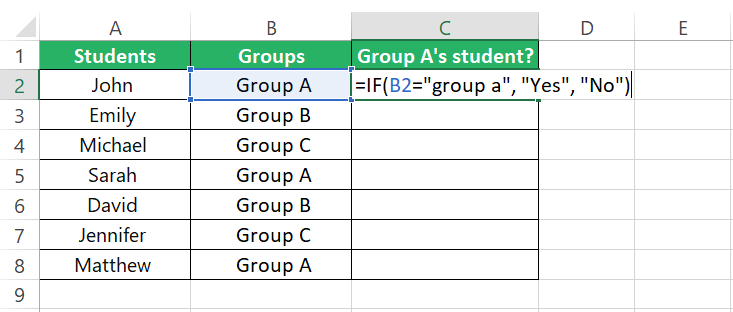
Step 4) Hit the enter button and drag the fill handle down to get results for the whole list.
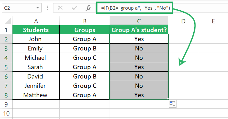
Excel checks each student to be from Group A and returns the results accordingly 📖
Check if the cell contains case-sensitive specific text
Notice that in the above section, the groups of students in the list were given as “Group A”, “Group B” and so on.
P.S: I am trying to draw your attention to the capital “G” and capital “A” 🅰
Whereas, in the IF function, I supplied the logical test as “group a” (with a small g and a).

Despite the difference in the case of “g”, the IF function returns TRUE and accordingly the value_if_true for all the cells that contain Group A. This proves that the IF function doesn’t account for case-sensitivity.
To check if a cell contains a case-sensitive specific text, we’d have to nest in the EXACT function in the IF function.
In the same student list as above, I have changed the case for some groups.
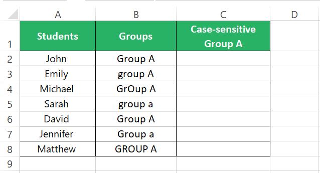
Now we only want Excel to return “Yes” for students whose group is written as “Group A” (with a capital G and A).
Step 1) Begin writing the IF function.
Step 2) For the logical test, we will use the EXACT function as below.
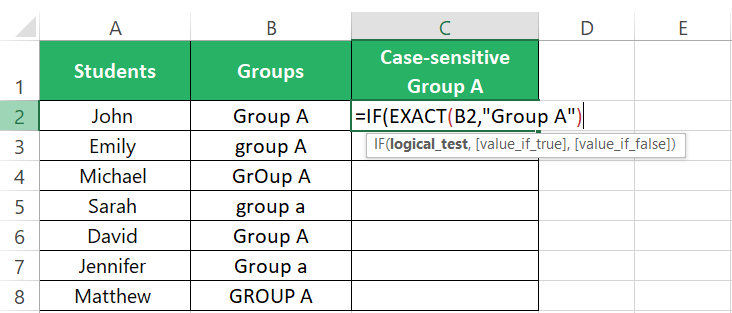
The EXACT function will check if the value in Cell B2 is exactly equivalent to “Group A” including the case of the letters.
Step 3) The rest of the function remains the same with the value_if_true and value_if_false.
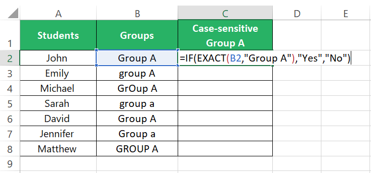
Step 4) Hit Enter and there you go.
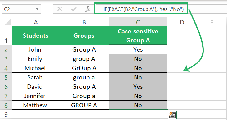
We only get a “Yes” for Cell B2 and B6. For all the other cells, it’s a “No”. This is how you can make Excel check for a case-sensitive value in a cell and get any value in return 🙈
Check if the cell contains a specific text string
The real search is about giving Excel a text string and making it find wherever that text string exists within the targeted cell.
Careful! We are talking about a text string and not about an entire text ⚠
For example, I have some email addresses populated in Excel below.
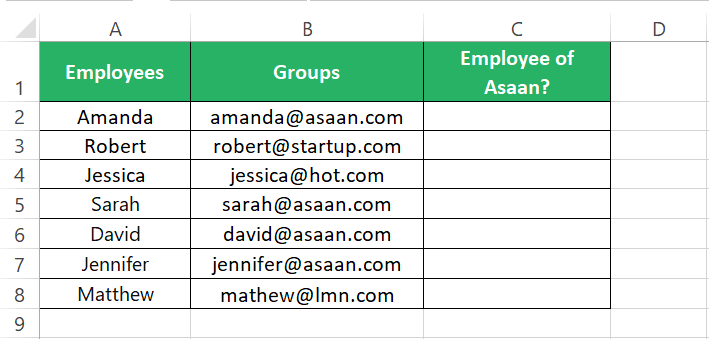
Each email is registered on a certain domain for example abc@asaan.com.
This tells that this email is associated with the domain name asaan.com which must be an organization/employer.
I now want to find employees from the domain name “asaan”.
For this, I need to tell Excel to check each email ID in the given cells and find out those that contain the text string “asaan”. The IF function will not help this situation as it looks out for complete text in a cell.
Whereas, what we are looking for is only a string from the text in the cells. No worries, here’s how we will take care of it 👇
Using the SEARCH function
Step 1) Write the SEARCH function as below.
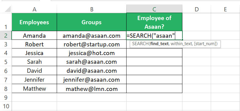
As the first argument, specify the text to be searched for.
Step 2) Then refer to the cell wherein the given text is to be looked for.
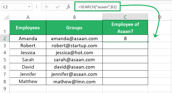
The SEARCH function looks for a text in a given cell and if the said text is found, it returns the number of characters from where onwards that text in the cell starts.
Step 3) Let me quickly drag this formula down to show you that for cells where the text “asaan” doesn’t exist, the SEARCH function returns a #VALUE! Error.
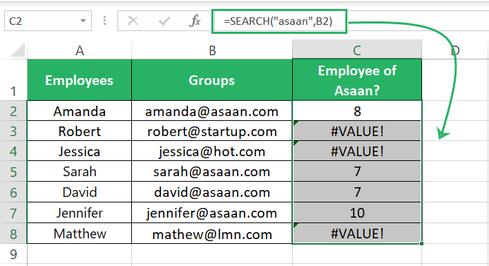
Step 4) Next, we will nest this function into the ISNUMBER function as below.
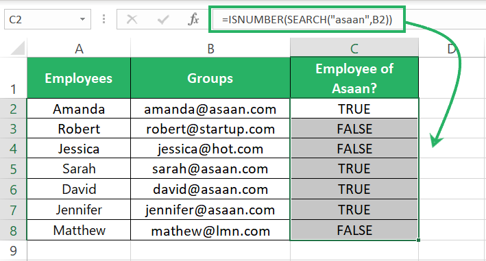
The ISNUMBER function is a logical function that checks if the given cell contains a number or not and returns the result as TRUE or FALSE. Just like the ISTEXT function checks for text.
So, we only get the result as “TRUE” for the cells that contain a number (which will be those where the text string “asaan” exists and the SEARCH function has returned the starting text string number for them).
Step 5) Nest the above function into the IF function to supply the desired value_if_true and value_if_false for the cells where the text string “asaan” exists and doesn’t exist, respectively.
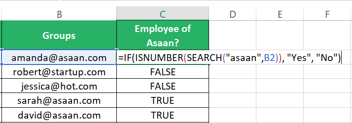
I have supplied “Yes” as the value_if_true and “No” as the value_if_false.
Step 6) Ready? Hit the enter button to have your results ready.
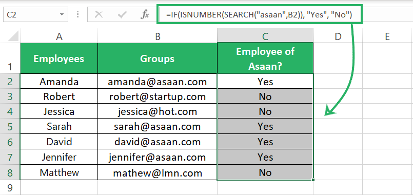
Together the IF, ISNUMBER, and SEARCH functions return a “Yes” for the email addresses that contain the text string “asaan” and “No” for those that do not.
Using the COUNTIF Function
The above results can also be achieved by using a combination of COUNTIF function and wildcard characters😃
Step 1) Write the COUNTIF function as below:
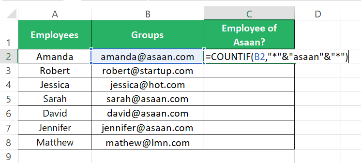
There are two asterisks (*) in inverted commas inserted with an ampersand (&) before and after the text string.
An asterisk is a wildcard character that tells Excel to look for the sandwiched text string (asaan) with any text preceding or succeeding it.
Step 2) Press Enter to see the results of the COUNTIF function.
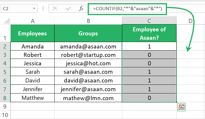
Note that where the referred cells contain the text string “asaan”, the COUNTIF function returns 1, and for the cells that do not, it returns 0.
In Excel, TRUE equals to “1” and FALSE equals to “0”.
Step 3) Nest the above function in the IF function and specify the value you want to be returned if the text string is found and if not found as the value_if_true and value_if_false.
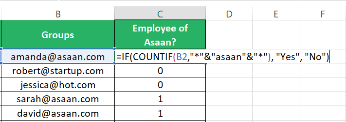
Step 4) Hit Enter and drag down the fill handle to see the following results.
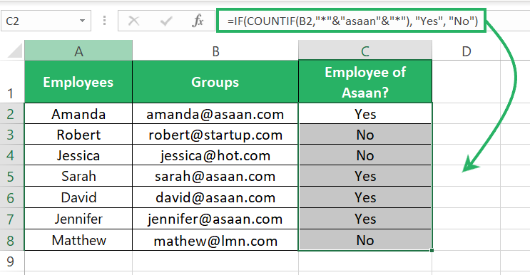
The SEARCH function and the COUNTIF function, both do not perform a case-sensitive search. If you need to yield results that take into account the case of the text string, see the section below.
Specific but case-sensitive text string
The SEARCH function will search for a given text string in a cell without catering to its case.
If you desire a case-sensitive search, the SEARCH function won’t work for you – but the FIND function will 🎯
To demonstrate this to you, I have changed the letter case of the text string “asaan” in the email addresses below.
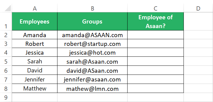
Both the functions are broadly the same with the difference that the FIND function accounts for the case of the given text string.
Let me show you here.
Step 1) Write the FIND function to search for the text string “asaan” (all letters in small) as follows.
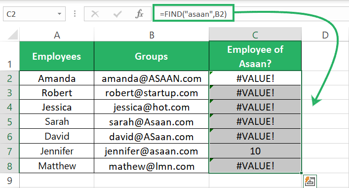
See the results? It returns a #VALUE! Error for all the cells except for C7 where the letter case of the given text string and the cell’s text exactly match.
Step 2) Everything else remains the same. Nest the above function into the ISNUMBER and then into the IF function as below.

Step 3) Hit enter to have case-sensitive results ready.
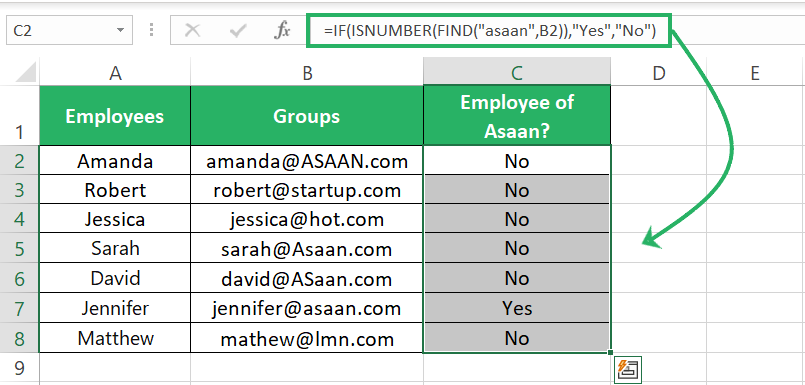
Note that this time, for a case-sensitive text string search, Excel returns the desired value only for Jennifer (where the case of the text string is an exact match) 👌
Conclusion
The guide above discusses several instances and circumstances to check if a cell contains text. And if it does, make Excel return a specific value.
Not only text, but you can also tweak the above formulas to check for other values. There are no limits to being innovative with Excel. Reading my below Excel tutorials will help you learn more about using some top-notch functions of Excel.
