How to Use the SEQUENCE Formula in Excel (Easy)
The SEQUENCE function in Excel allows you to automatically generate a sequence of numbers or dates. You can create a simple sequence or a custom sequence with increments of your choice.
SEQUENCE function offers an easy way to streamline your data and boost your efficiency when working in an Excel spreadsheet 📗
Let’s see a detailed explanation of the SEQUENCE function in the tutorial below where we break down its syntax and see different use cases and practical examples.
Download our sample workbook here to practice along with us 🧐
Excel SEQUENCE formula
Excel SEQUENCE function allows you to generate arrays of sequential numbers in no time. This is very useful if you want to create a numbered list for some data or want to create grids of different shapes and sizes ⬛
SEQUENCE is a dynamic array function which means that depending on the arguments, it fills in the columns and rows automatically.
Its syntax is explained below:
where,
rows refers to the number of rows you want to fill
column refers to the number of columns to fill – where its default value is 1
start refers to the number where the sequence starts from – with the default value as 1
step refers to an increment in each value to appear in the sequence -its default value is 1 and it can be positive or negative where the subsequent values increase or decrease.
Note that the SEQUENCE function is only available in MS Excel 365 and 2021 versions. That is because SEQUENCE is a dynamic array function and any version before Excel 2021 doesn’t support dynamic array formulas.
Creating a number sequence in Excel
The simplest use case of the SEQUENCE function is to populate your rows and columns with sequential values. Let’s see how to do that below 🔽
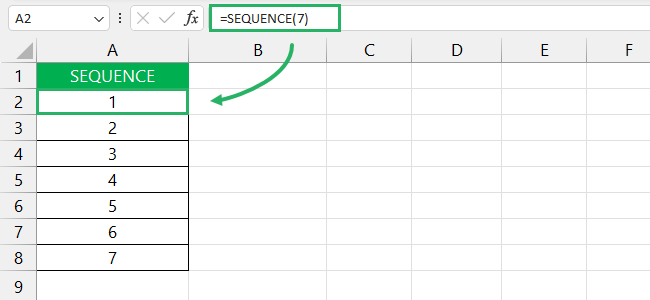
Say, in a sheet I want 7 sequential values in one column.
To do that,
Step 1) Select a cell.
Step 2) Type in the following formula.
Step 3) Press Enter.
The SEQUENCE formula would return a row of values from 1 – 7. This creates a one-dimensional array that holds the values of a column.
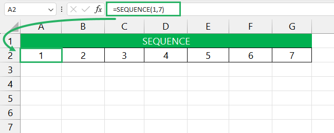
To place numbers in a single row, change the arguments (1, n) as:
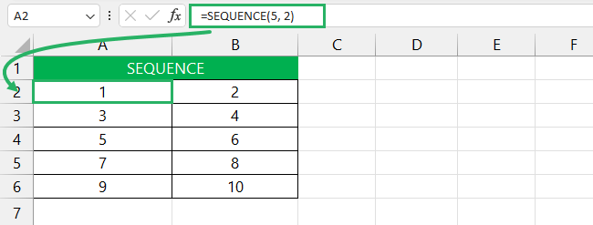
Similarly, if you want to create a grid, supply both arguments as:
This would return 10 values as 5 x 2 —> (rows x columns) in a two-dimensional array – you only need to add two parameters for that 2️⃣
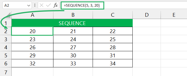
You can also choose a different start value for your sequence list by providing a value to the start parameter as (5, 3, 20). Your list of sequential numbers then begins at 20.
If you want to customize the increment value of your sequence, you can set that in the step parameter of the function as (5, 3, 1, 2). This will show you a grid of odd numbers as:
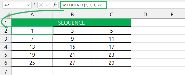
Or you could do the same in decreasing order using parameters like (5, 3, 20, -2). This will return odd values starting from 20 in decreasing order.
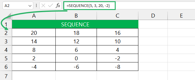
An important thing to note is that the SEQUENCE function in Excel outputs all the values in a spill range. This means the cell where you input the formula should have empty cells on its right and bottom.
Otherwise, the function will throw a #SPILL error and you will have to either remove values in the neighbouring cells or paste the formula elsewhere in the worksheet ⚠
Excel SEQUENCE formula examples
Let’s look at a couple of examples of the SEQUENCE function in combination with other functions below.
TRANSPOSE Function
SEQUENCE function is often used in combination with the TRANSPOSE function in Excel. It lets you change the order and even the shape of the grid depending on the order of the arguments.
We use SEQUENCE function with TRANSPOSE as:
Note that the rows and columns argument has been switched here – this is to swap the order of the values 🔁
Let’s see its use case below.
Step 1) Select a cell.
Step 2) Type in the following formula.
Step 3) Press Enter.
The function returns a matrix as:
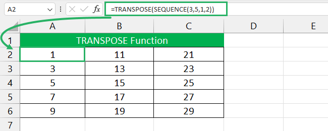
To see the difference between a transposed grid and a normal SEQUENCE-generated grid, see the screenshot below 📷
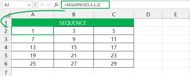
In the SEQUENCE function, the values appeared in a left-to-right order, i.e., horizontally. After applying TRANSPOSE, the values now appear in a top-to-bottom order, i.e., vertically.
But note that the shape of the grid remains the same. If you want to change the shape of the grid, swap the row and column arguments as:
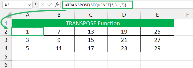
The grid shows values in the top to bottom order but its shape and size have now changed. The difference won’t be visible if you are dealing with a square matrix 🟨
Date Function
Another popular use case of the SEQUENCE function is with the DATE function. Sometimes you need to generate the dates of months quickly and typing them manually is not an option.
Let’s use it with the SEQUENCE function.
Step 1) Select any cell.
Step 2) Type in the following formula.
Step 3) Press Enter.
It will return the result as:
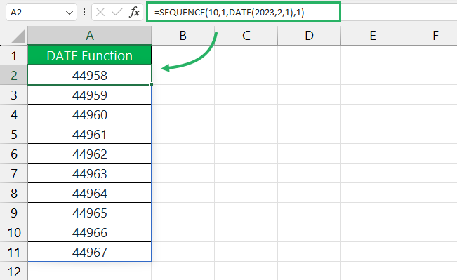
These are dates but in number format which gives the impression the data makes no sense. To fix it, select all the values, go to the General bar under the Number section and select Short Date 📆
You can customize your date format too by going to custom and typing in your custom format. We changed it to d-m-yy by setting a custom preference.
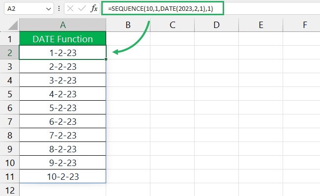
You can also use the TODAY function in combination as:
Apply the same format as above from the Number section on the Home tab to get the sequence of dates:
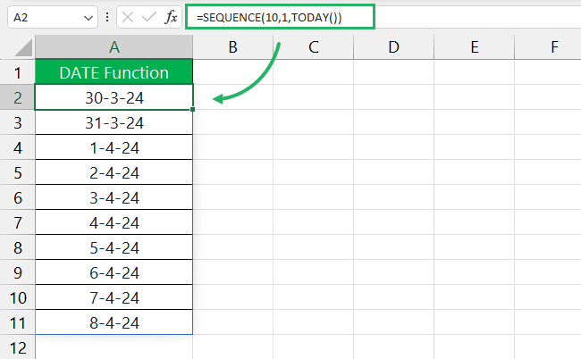
Using SORTBY Function to generate random values
We use the RANDARRAY function in combination with the SORTBY and SEQUENCE function to create a random list of numbers. You can modify the formula to give you increasing or decreasing values.
Let’s see how this works below.
Step 1) Select a cell.
Step 2) Type in the following formula.
Step 3) Press Enter.
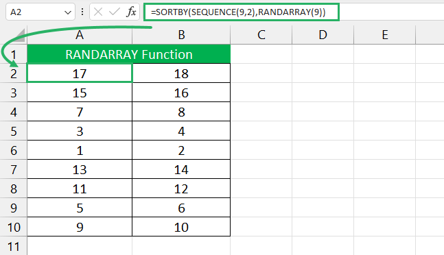
The formula generates a matrix of 9 x 2, returns an array of 18 values and sorts it according to the 9 elements returned by the RANDARRAY function.
Note that we are using the same size for RANDARRAY as the SEQUENCE function’s row argument. This is to pair each element in the array generated by SEQUENCE with a random number from the RANDARRAY result.
This pairing is crucial for the SORT function to sort rows based on random numbers. If you were to provide different parameters for both, you would encounter a #VALUE! error ⚠
This is because the SORTBY function wouldn’t have any corresponding random number for each row of the SEQUENCE function.
If you were to decrement the values by the same margin, you would simply add a minus sign before the RANDARRAY function as in the formula below 🔽
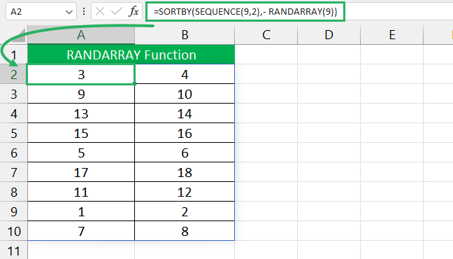
Using COUNTA Function
If you want to create a list of numbers equal to the number of entries in the adjacent list, the COUNTA function is exactly what you need 😃
It counts the text values in the neighbouring column and returns an array of sequential numbers where the count is the number of rows in the SEQUENCE function. Let’s see how to use it below.
Step 1) Select a cell.
Step 2) Type in the following formula ⌨
Step 3) Press Enter.
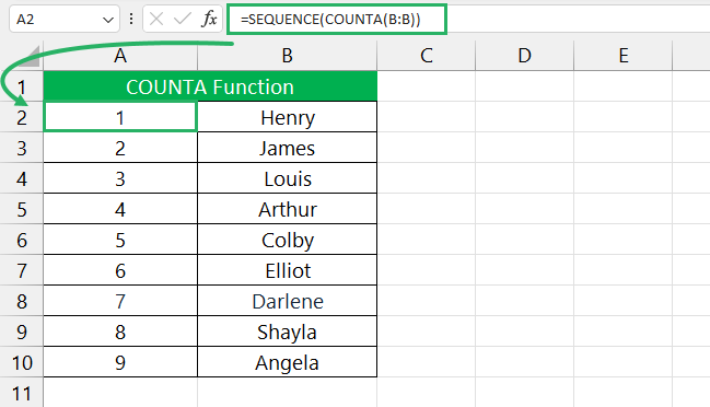
This counts all the values in column C and creates the sequence according to the count. You can also CONCATENATE different words with the list. To do that, use the formula below.
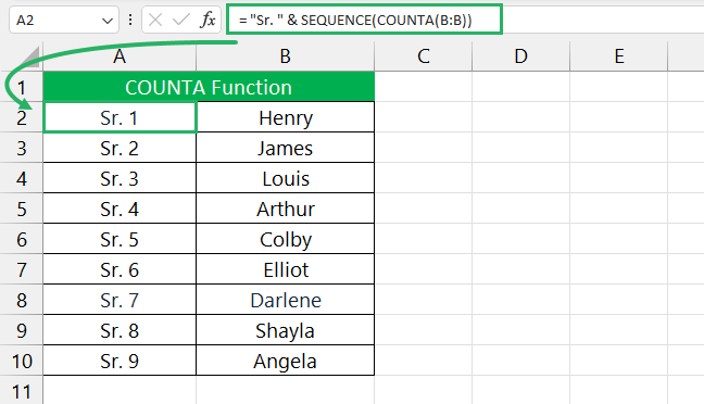
Conclusion
In this article, we saw how the SEQUENCE function works, its different use cases and formula examples. SEQUENCE function is extensively used in data analysis and manipulation.
It can be a lifesaver in times when Fill Handle isn’t giving you the desired results for a list of numbers dates or even text strings as it keeps changing ☹
You can learn more about SEQUENCE and other functions in Microsoft Excel using the links below.
How to Fix the #Spill Error in Excel (Step-by-Step)
How to Randomize a List in Excel: Step-By-Step Guide (2024)
Today’s Date in Excel: Function and Formula Examples (2024)
We hope you enjoyed reading this article as much as we did creating it.
